
Introduction to Equilibrium
Introduction to Equilibrium
What you’ll learn to do: explain market equilibrium, surplus, and shortage
In this section, we’ll put the two fundamental pieces of the economic puzzle—supply and demand—together and see how the two laws interact in market situations. This section also introduces the concept of equilibrium—a stable market condition—and illustrates situations where the market is out of equilibrium, resulting in either a short-term surplus or shortage situation, and the resulting market pressure toward equilibrium. Finally, this section provides opportunities to work through scenarios where market factors result in shifts in both supply and demand.
1. Surpluses and Shortages
LEARNING OUTCOMES
- Explain surpluses and shortages
In order to understand market equilibrium, we need to start with the laws of demand and supply. Recall that the law of demand says that as price decreases, consumers demand a higher quantity. Similarly, the law of supply says that when price decreases, producers supply a lower quantity.
Because the graphs for demand and supply curves both have price on the vertical axis and quantity on the horizontal axis, the demand curve and supply curve for a particular good or service can appear on the same graph. Together, demand and supply determine the price and the quantity that will be bought and sold in a market. These relationships are shown as the demand and supply curves in Figure 1, which is based on the data in Table 1, below.
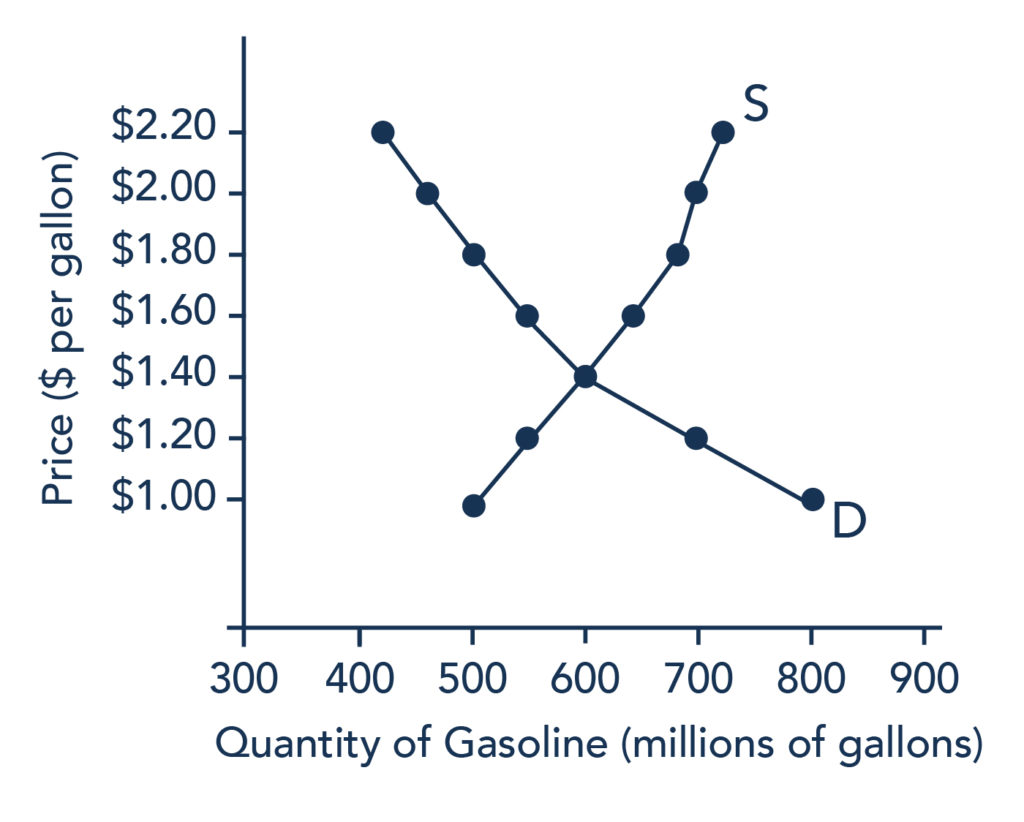
Figure 1. The supply and demand curves for gasoline.
| Price (per gallon) | Quantity demanded (millions of gallons) | Quantity supplied (millions of gallons) |
|---|---|---|
| $1.00 | 800 | 500 |
| $1.20 | 700 | 550 |
| $1.40 | 600 | 600 |
| $1.60 | 550 | 640 |
| $1.80 | 500 | 680 |
| $2.00 | 460 | 700 |
| $2.20 | 420 | 720 |
If you look at either Figure 1 or Table 1, you’ll see that at most prices, the amount that consumers want to buy (which we call the quantity demanded) is different from the amount that producers want to sell (which we call the quantity supplied). What does it mean when the quantity demanded and the quantity supplied aren’t the same? The answer is: a surplus or a shortage.
Surplus or Excess Supply
Let’s consider one scenario in which the amount that producers want to sell doesn’t match the amount that consumers want to buy. Consider our gasoline market example. Imagine that the price of a gallon of gasoline were $1.80 per gallon. This price is illustrated by the dashed horizontal line at the price of $1.80 per gallon in Figure 2, below.
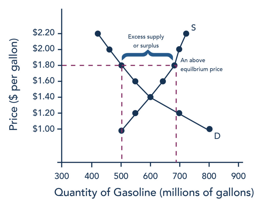
Figure 2. A price above equilibrium creates a surplus.
At this price, the quantity demanded is 500 gallons, and the quantity of gasoline supplied is 680 gallons. You can also find these numbers in Table 1, above. Now, compare the quantity demanded and quantity supplied at this price. Quantity supplied (680) is greater than quantity demanded (500). Or, to put it in words, the amount that producers want to sell is greater than the amount that consumers want to buy. We call this a situation of excess supply (since Qs > Qd) or a surplus. Note that whenever we compare supply and demand, it’s in the context of a specific price—in this case, $1.80 per gallon.
With a surplus, gasoline accumulates at gas stations, in tanker trucks, in pipelines, and at oil refineries. This accumulation puts pressure on gasoline sellers. If a surplus remains unsold, then those firms involved in making and selling gasoline are not receiving enough cash to pay their workers and cover their expenses. In this situation, some firms will want to cut prices, because it is better to sell at a lower price than not to sell at all. Once some sellers start cutting prices, others will follow to avoid losing sales. These price reductions will, in turn, stimulate a higher quantity demanded.
How far will the price fall? Whenever there is a surplus, the price will drop until the surplus goes away. When the surplus is eliminated, the quantity supplied just equals the quantity demanded—that is, the amount that producers want to sell exactly equals the amount that consumers want to buy. We call this equilibrium, which means “balance.” In this case, the equilibrium occurs at a price of $1.40 per gallon and at a quantity of 600 gallons. You can see this in Figure 2 (and Figure 1), where the supply and demand curves cross. You can also find it in Table 1 (the numbers in bold).
Shortage or Excess Demand
Let’s return to our gasoline problem. Suppose that the price is $1.20 per gallon, as the dashed horizontal line at this price in Figure 3, below, shows. At this price, the quantity demanded is 700 gallons, and the quantity supplied is 550 gallons.
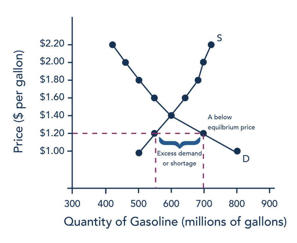
Figure 3. A price below equilibrium creates a shortage.
Quantity supplied (550) is less than quantity demanded (700). Or, to put it in words, the amount that producers want to sell is less than the amount that consumers want to buy. We call this a situation of excess demand (since Qd > Qs) or a shortage.
In this situation, eager gasoline buyers mob the gas stations, only to find many stations running short of fuel. Oil companies and gas stations recognize that they have an opportunity to make higher profits by selling what gasoline they have at a higher price. These price increases will stimulate the quantity supplied and reduce the quantity demanded. As this occurs, the shortage will decrease. How far will the price rise? The price will rise until the shortage is eliminated, and the quantity supplied equals quantity demanded. In other words, the market will be in equilibrium again. As before, the equilibrium occurs at a price of $1.40 per gallon and at a quantity of 600 gallons.
Generally any time the price for a good is below the equilibrium level, incentives built into the structure of demand and supply will create pressures for the price to rise. Similarly, any time the price for a good is above the equilibrium level, similar pressures will generally cause the price to fall.
As you can see, the quantity supplied or quantity demanded in a free market will correct over time to restore balance, or equilibrium.
2. Equilibrium, Price, and Quantity
LEARNING OUTCOMES
- Explain equilibrium price and quantity
Equilibrium: Where Supply and Demand Intersect
When two lines on a diagram cross, this intersection usually means something. On a graph, the point where the supply curve (S) and the demand curve (D) intersect is the equilibrium. The equilibrium price is the only price where the desires of consumers and the desires of producers agree—that is, where the amount of the product that consumers want to buy (quantity demanded) is equal to the amount producers want to sell (quantity supplied). This mutually desired amount is called the equilibrium quantity. At any other price, the quantity demanded does not equal the quantity supplied, so the market is not in equilibrium at that price. It should be clear, from the previous discussions of surpluses and shortages, that if a market is not in equilibrium, then market forces will push the market to the equilibrium.
If you have only the demand and supply schedules, and no graph, then you can find the equilibrium by looking for the price level on the tables where the quantity demanded and the quantity supplied are equal (again, the numbers in bold in Table 1 indicate this point).
FINDING EQUILIBRIUM WITH ALGEBRA
We’ve just explained two ways of finding a market equilibrium: by looking at a table showing the quantity demanded and supplied at different prices, and by looking at a graph of demand and supply. We can also identify the equilibrium with a little algebra if we have equations for the supply and demand curves. Let’s practice solving a few equations that you will see later in the course. Right now, we are only going to focus on the math. Later, you’ll learn why these models work the way they do, but let’s start by focusing on solving the equations. Suppose that the demand for soda is given by the following equation:
where Qd is the amount of soda that consumers want to buy (i.e., quantity demanded), and P is the price of soda. Suppose the supply of soda is
where Qs is the amount of soda that producers will supply (i.e., quantity supplied). (Remember, these are simple equations for lines). Finally, recall that the soda market converges to the point where supply equals demand, or
We now have a system of three equations and three unknowns (Qd, Qs, and P), which we can solve with algebra. Since
we can set the demand and supply equations equal to each other:
Step 1: Isolate the variable by adding 2P to both sides of the equation and subtracting 2 from both sides.
Step 2: Simplify the equation by dividing both sides by 7.
The equilibrium price of soda, that is, the price where Qs = Qd, will be $2. Now we want to determine the quantity amount of soda. We can do this by plugging the equilibrium price into either the equation showing the demand for soda or the equation showing the supply of soda. Let’s use demand. Remember, the formula for quantity demanded is the following:
Taking the price of $2, and plugging it into the demand equation, we get
So, if the price is $2 each, consumers will purchase 12. How much will producers supply, or what is the quantity supplied? Taking the price of $2, and plugging it into the equation for quantity supplied, we get the following:
Now, if the price is $2 each, producers will supply 12 sodas. This means that we did our math correctly, since
s
and both Qd and Qs are equal to 12. That confirms that we’ve found the equilibrium quantity.
WATCH IT
Watch this video for a closer look at market equilibrium:
You can view the transcript for “Episode 14: Market Equilibrium” (opens in new window).
Equilibrium occurs at the point where quantity supplied = quantity demanded.
Equilibrium and Economic Efficiency
Equilibrium is important to create both a balanced market and an efficient market. If a market is at its equilibrium price and quantity, then it has no reason to move away from that point, because it’s balancing the quantity supplied and the quantity demanded. However, if a market is not at equilibrium, then economic pressures arise to move the market toward the equilibrium price and equilibrium quantity. This happens either because there is more supply than what the market is demanding, or because there is more demand than the market is supplying. This balance is a natural function of a free-market economy.
Also, a competitive market that is operating at equilibrium is an efficient market. Economists typically define efficiency in this way: when it is impossible to improve the situation of one party without imposing a cost on another. Conversely, if a situation is inefficient, then it becomes possible to benefit at least one party without imposing costs on others.
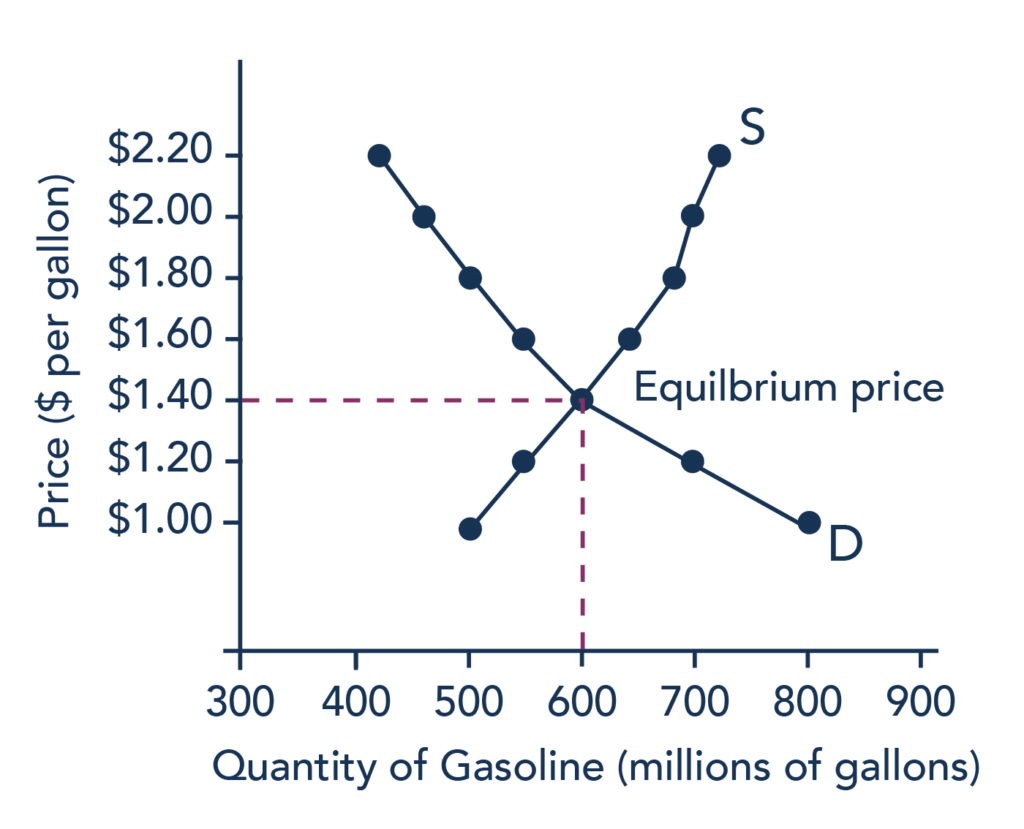
Figure 2. Demand and Supply for Gasoline: Equilibrium. At this equilibrium point, the market is efficient because the optimal amount of gasoline is being produced and consumed.
Efficiency in the demand and supply model has the same basic meaning: the economy is getting as much benefit as possible from its scarce resources, and all the possible gains from trade have been achieved. In other words, the optimal amount of each good and service is being produced and consumed.
Finding Equilibrium Using the Four-Step Process
We know that equilibrium is the place where the supply and demand curves intersect, or the point where buyers want to buy the same amount that sellers want to sell. Let’s take a closer look at how to find the equilibrium point using the four-step process. These steps explain how to first draw the demand and supply curves on a graph and find the equilibrium. Next, consider how an economic change (e.g., a natural disaster, a change in production technology, a change in tastes and preferences, income, etc.) might affect supply or demand, then make adjustments to the graph to identify the new equilibrium point.
Step 1. Draw demand and supply curves showing the market before the economic change took place. Think about the shift variables for demand, and the shift variables for supply. Using this diagram, find the initial equilibrium values for price and quantity.
Step 2. Decide whether the economic change being analyzed affects demand or supply. In other words, does the event refer to something in the list of demand shift variables or supply shift variables?
Step 3. Determine whether the effect on demand or supply causes the curve to shift to the right or to the left, and sketch the new demand or supply curve on the diagram. In other words, does the event increase or decrease the amount consumers want to buy or the amount producers want to sell?
Step 4. Identify the new equilibrium, and then compare the original equilibrium price and quantity to the new equilibrium price and quantity.
Try It
Play the simulation below multiple times to see how different choices lead to different outcomes. All simulations allow unlimited attempts, so that you can gain experience applying the concepts.
- Episode 14: Market Equilibrium. Authored by: Dr. Mary J. McGlasson. Located at: https://youtu.be/W5nHpAn6FvQ?t=1s. License: CC BY-NC-ND: Attribution-NonCommercial-NoDerivatives
- Supply, and Equilibrium in Markets for Goods and Services. Authored by: OpenStax College. Located at: https://cnx.org/contents/aWGdK2jw@11.346:D3bzsNhU@8/Demand-Supply-and-Equilibrium-. License: CC BY: Attribution. License Terms: Download for free at http://cnx.org/contents/4061c832-098e-4b3c-a1d9-7eb593a2cb31@11.11
- Principles of Macroeconomics Chapter 3.3. Authored by: OpenStax College. Provided by: Rice University. Located at: http://cnx.org/contents/ea2f225e-6063-41ca-bcd8-36482e15ef65@10.31:24/Microeconomics. License: CC BY: Attribution. License Terms: Download for free at http://cnx.org/content/col11627/latest