
Keynesian Macroeconomic Theory
Why Should I Care?
Politicians spend your money. You might want to understand what their arguments are for increasing expenditures, or changing tax rates. Hint: most of their arguments come from Keynes’ macroeconomic theory.
This Lecture Has 8 Parts
- Sorting Out the Variables
- The Keynesian Cross
- Unemployment and Equilibrium
- Shifts in AE
- Limitations
- Solving for Equilibrium
- The Government Multiplier
- Principles
What is Keynesian Macroeconomic Theory?
There are dozens of macroeconomic theories, and most of them stem from the models inspired by J. M. Keynes’ famous theory about aggregate demand (published in 1936). We will present here the basic ideas of the macroeconomic model known as the “Keynesian Cross.” This model was first drawn not by Keynes, but by Paul Samuelson and William Nordhaus in 1948. John Hicks is widely credited with the first graphical version, now called IS-LM, in 1937.
The model has two main objectives. The first one is to explain how a certain level of aggregate economic activity can be insufficient to create employment for everyone in society. The model therefore offers an argument for government intervention to step in and provide stimulus to the economy. The second objective is to quantify the amount of government expenditure required to fill in an output gap.
Hence, Keynesian economics provides a rationale for interventionism.
This argument echoes the widely-held view at the time (1930's), that there would always be enough demand to justify a given level of supply. This principle is called Say's Law, and was formulated by French economist Jean-Baptiste Say in 1803. The basic idea is actually hard to translate to English. It is called the ''Loi des débouchés'', which in English means other avenues, or market opportunities. Say wrote that the production of a good generates the opportunity to purchase other goods. Over time, the principle was used to understand the general equilibrium between aggregate demand and aggregate supply of goods and services. The principle also states that supply generates demand, and so it is associated to pro-industry views. Prior to Keynes, many economists were proponents of Say's Law, especially the marginalists such as Leon Walras, Carl Menger and Alfred Marshall.
The Keynesian view does not contradict Say's Law directly, it adds an interesting twist: this equilibrium of demand and supply may be insufficient to provide enough employment for the population. The Keynesian view was therefore a full-frontal attack on marginalist laissez-faire economics, whose lack of reaction to the suffering of people during the Great Depression (1929-1939) prompted Keynes to argue for government intervention. In Britain, the keynesian economists were known as the Cambridge school, while the marginalist
-
Sorting Out the Variables
First of all, we must identify the variables in the model, and associate each to a role. This will help us sort out the relationships between the variables and how they will be used in the model, which, I remind you, is a simulation of what the economy could really be like.
Keynes’ basic idea was to explain the level of employment, with the level of output. These are the two most important variables. In its essence, Keynes argued that employment is determined by output, which is determined by aggregate demand. In short, aggregate demand (AD) is a function of consumption, government spending, and investments.
Diagram - Aggregate demand drives Output and Employment
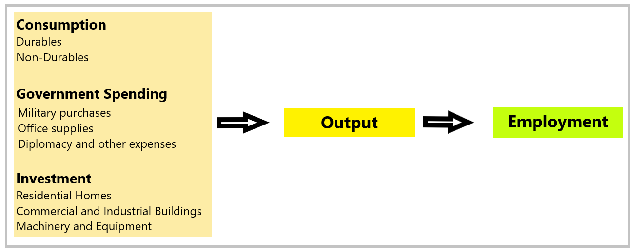
Each of the components of AD has its behaviour and root causes. Consumption is a function of the rate of savings, wealth, and wage rates. Government spending is a function of tax revenue and the projects at hand. Investment is dependent on interest rates and the level of savings stocked in bank accounts.
This keynesian linear explanation was in fact in opposition to the marginalist view that output was the initial driver of aggregate demand, and that employment levels would adjust with swift wage variations. This view also posits that savings and investments are constantly adjusting to each other.
Keynes disagreed with this view for a few reasons. First, he argued that labour markets cannot constantly be clearing, due to the difficulty of actually changing wages swiftly. He called this sticky wages. Second, he had observed that investment levels did not always match savings, because investors may behave in cycles. Keynes went so far as to say that investors don't always act rationally, using the term animal spirits. When the economy is doing well, investments may be more important than savings. More importantly, when the economy is slow, investors tend to by shy and hold on to their savings rather than spend them on a risky project.
The conclusion of Keynes theory, is that in general, employment is insufficient to provide the entire labour force with a meaningful well-paid job. This is why he titled his book, The General Theory of Employment, Interest and Money. Keynes argument is that the level of production in the economy does not always match a situation of equilibrium between the aggregate level of spending in the economy, and the aggregate level of income. According to Keynes there can be a situation of entrenched unemployment.
To build the model, we actually take employment out of the equations. We will assume that employment is directly related to output. Any change in output is positively associated to a change in employment.
To understand Keynes' theory, you have to imagine that output, which is a flow, can be determined two ways. The first to determine the supply side. We will graph aggregate supply on the horizontal axis. Some textbooks call it Aggregate supply, other texts call it Output (Y), or Aggregate income. We will use Y.
Next is aggregate demand, which can also be called Aggregate expenditure (AE). We will measure AE on the vertical axis.
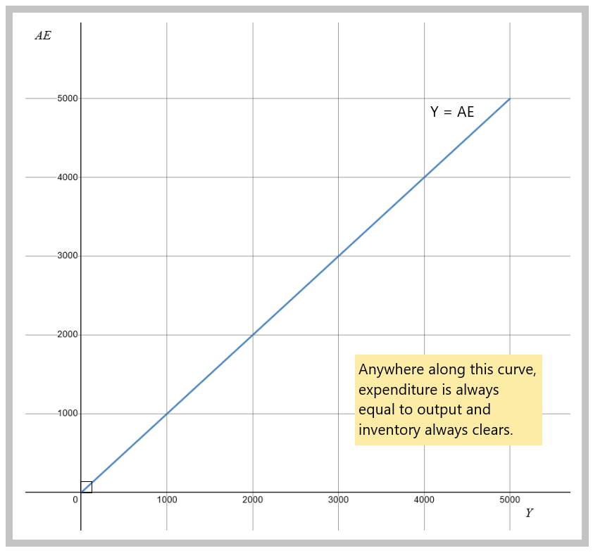
Y = AE curve
The model starts with a design where a any level of aggregate production would represent an equilibrium of aggregate demand and output. At equilibrium, we have an equality between output and expenditure, where:
Y = AE
The Y = AE curve is the visual representation of the circular flow diagram, where all of the expenditures are equal to incomes. It also represents the marginalist view of Say's Law, where supply always generates enough demand for its output.
AE curve
The AE curve has a slow and positive slope and starts rather high on the intersect. It will cross the Y = AE curve at a single coordinate on the graph.
The AE curve is made up of three main components, consumer spending, government spending, and investment spending. If you want to include international trade, you can add net exports.
Aggregate Expenditure = Consumer spending + Government spending + Investment spending + Net Exports
AE = C + G + I + (X-M)
What all of this means is that our level of production depends on spending. But if aggregate spending does not equal income, the system will be out of balance. The model illustrates situations when spending does not match income, which results in entrenched unemployment.
About Prices.
The model does not discuss price levels in relation to AE or output. Original Keynesians take price levels to be fixed. In this model, the dependent variable is Y, the level of production. All of the other variables are independent, such as income, expenditure, and any environmental variables such as productivity, technology, demographics, etc.
Does dual-entry accounting solve the riddle?
You already know that GDP is measured using dual-entry accounting. Each transaction is sorted into either an expenditure account, or an income account. The sum of both sides must be equal. This measurement of output is considered actual output. Keynesian theory defines AE and Y as planned expenditures, and planned output, rather than actual. It is the difference between the plans of the spenders (AE) and the plans of the producers (Y), that explain why there could be difference between both variables.
What explains output?
The dependent variable of the model is Y, output. The point is to get aggregate output back to potential and solve the problem of unemployment. The variables that explain changes in output are part of the demand-side of the economy. We divide them into two categories: endogenous (effects predicted by the model), and exogenous (prior cause).
AE is an endogenous aggregate, made up of the variables C, G, I, and X-M.
C is assumed to have two components. First, an autonomous level of expenditure which is not related to income levels. This base of consumption is constant, even if income were to be nil. This is possible because consumption is a flow which can be fed from stocks of savings, or the creation of new loans.
Second, C also varies with income, which is called induced consumption. The rate at which C increases due to income is called the Marginal Propensity to Consume, and is considered to be a constant share of new income. It's slope is therefore linear and constant.
G, I, and X-M, are assumed to be fixed, and unrelated to income. They are considered autonomous. The sum of the autonomous expenditures determines the intersect of the AE curve on the horizontal axis.
Exogenous factors can affect the variables in the model. For example, a sudden increase in population can shift the C, G, and I variables higher, moving the autonomous level up the horizontal axis, and moving the whole curve up.
-
The Keynesian Cross
The first thing we need to draw is what Keynesians call the 45 degree line. This curve represents all the levels of production at equilibrium, where AE = Y. This line is used as a benchmark.
The Y = AE curve is a perfect 45 degree curve and its coordinates always form a perfect box. For example, if Y = 1.5 T$, then so does AE on the 45 degree curve. This coordinate (1.5 T$, 1.5 T$), indicates that this level of demand is also supplied to markets.
The AE = Y curve is infinite, as we are discussing a scenario where labour is not scarce. However, as you will see, the model is intended to be used to analyze situations where output is below potential. The model is designed to discuss situations when at least some resources are idle, indefinitely, such as an economic depression. The model is not designed to discuss overproduction, which is a major environmental issue we should discuss later.
Graph - The 45 Degree Curve (figures in B$)
The next thing we need to draw is the AE curve, which is the sum of C, G, I, and X-M. This one is trickier.
First, we assume that spending will never be zero, even if income is zero. Why? The model assumes that a society can use savings, or loans, to consume at a minimal level to avoid starvation and death. This is called the autonomous level of expenditure. By the way, this is exactly what happened during the COVID-19 pandemic, when many people used savings to continue paying for rent and groceries. The government used public debt to help those who lost income and had no savings.
We will note autonomous consumption as Ca and induced consumption as Ci. The other components are solely autonomous, so their notation does not need to be modified.
Aggregate expenditure = AE = Ca + Ci + G + I + (X-M)
So let’s scale and set autonomous expenditure at 1,200 billion dollars (1.2 trillion), on the AE axis (vertical).
The next step is to include the induced expenditures. This spending is a function of income. As income rises, we spend more. For each dollar of added income, AE will rise. But. There are savings and other withdrawals from the system such as personal income tax and spending on imports. For the sake of this introductory text, let's consider only the savings aspect.
We will note induced consumption as Ci. Consumers don’t spend the whole dollar of their extra income. If their savings rate is 30 percent, they will spend 70 cents on the dollar. Because of savings, the slope of the AE curve cannot be as steep as the 45 degree curve. For example, the marginal propensity to consume can be 70%.
if, MPC = 0.7
and, Ci = MPC*Income
then: Ci = 0.7*Y
Since the MPC is the slope of the curve, and that the slope is smaller than 1, but greater than 0, the two curves will therefore cross. This cross-point represents the equilibrium level of production.
Graph - Where AE meets the 45 Degree Curve
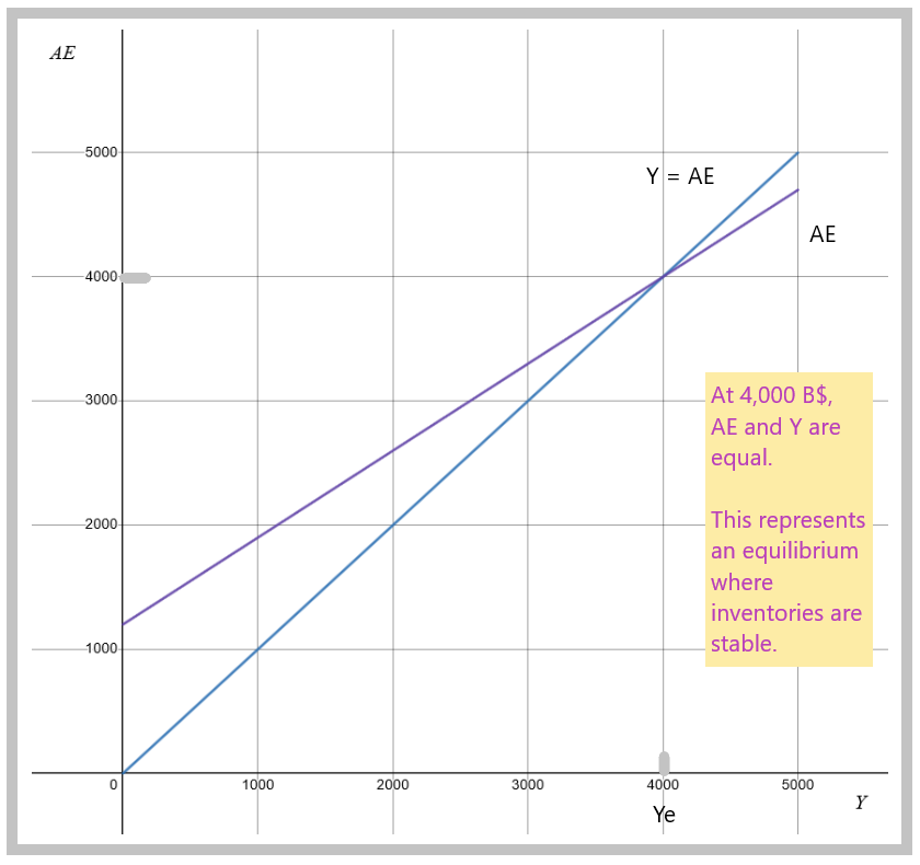
As you can see on the graph, the AE curve's intersect is at (1200, 0), representing autonomous expenditures. The curve then proceeds on a positive slope, due to the income-induced expenditures. The AE curve crosses the Y = AE curve at (4000, 4000). The equilibrium level of output is therefore given at Y = 4,000 B$, or 4.0 trillion dollars. This is roughly twice the size of the Canadian economy. Notice the scales of the Y axis, and the AE axis are identical. This is on purpose. The equilibrium coordinate (4000, 4000) forms a perfectly square box, hence the 45 degree angle of the Y = AE curve.
Macroeconomic equilibrium is maintained by a simple feedback mechanism: inventories. If you choose a point on the AE curve which is superior to Y, this represents a situation where inventories are depleted. For example, at AE = 3,720 B$, and Y = 3,600 B$. Output would be insufficient to supply the demand. This would prompt suppliers to increase production, so the coordinate on the AE curve achieves the level where Y = AE.
Graph - Inventories Balance the Macro Economy
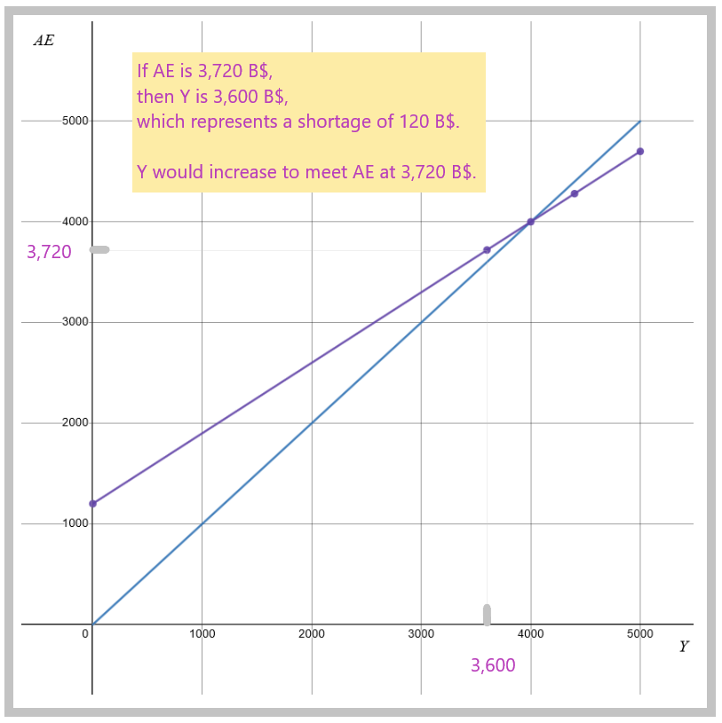
When AE is inferior to Y, inventories in excess and accumulate on the shelves. For example, at AE = 4,280 B$, and Y = 4,400 B$. Output would be too high for the level of demand. This prompts suppliers to decrease production, until Y = AE.
The inventory feedback may explain small and short-lived recessions. These situations are temporary and will return to normal. Hence, the Keynesian model does allow for free markets to self-regulate if the difference between production and aggregate expenditure are not great.
Also, at equilibrium, Investments are equal to savings, or I = S. If not at equilibrium, the difference between AE and Y implies that there is a level of dissaving (or oversaving), where S is smaller (or larger) than I. This aspect of the model is explained in more detail in more advanced texts.
-
Unemployment and Equilibrium
Unemployment may exist even if the system is in equilibrium. This statement put Keynes at odds with the Classical school of thought, epitomized by Adam Smith, and later Jean-Baptiste Say. According to Say's Law, employment income is always sufficient to purchase all of the production in the economy.
Keynes argued that during an important recession, or worse a depression, sometimes planned production is larger than sales. Capitalists and industrialists can mistakenly estimate consumer demand. Let's say workers have been paid to make automobiles, but only 90 percent of output has been sold in that year. Management has to reduce planned output by more than the 10 percent missing, because they need to sell the overstock before they can bring production levels back to regular levels. This mismatch between planned output and planned expenditures is not accounted for in classical economics.
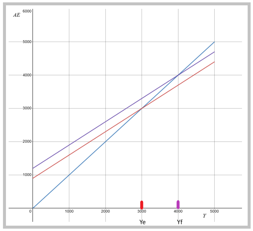
To establish this on the graph, you have to identify the production level associated to full-employment (Yf). You then compare that level of production with the equilibrium level of production (Ye).
If Yf > Ye , there is an under-production output gap
If Yf < Ye , there is an n you have an over-production output gap.
This aspect of the model is referred to Entrenched Unemployment. This concept is associated to deeper and long-lived recessions, the worse of which are called depressions. In these cases, the simple inventory feedback will be insufficient. The output gap is much larger, and is due to a drop in autonomous (planned) expenditures. When this is the case, government intervention is argued for by Keynesian economists.
The graph below shows a situation where the economy is severely depressed. The AE curve dropped to a new position, and a new equilibrium has emerged. The red mark represents Ye, a much lower level of production than the previous equilibrium, which is illustrated by the purple mark representing Yf, the desired level of output to achieve full employment. If you look at the Y axis, you will notice the difference is worth 1,000 billion dollars in GDP.
Graph - Visualizing Entrenched Unemployment
According to keynesians, the solution to generate more employment, is to stimulate the economy using government expenditure.
Play with the Graph
You can play around with the curves on Desmos. Click below.
-
Shifts in AE
The tragic problem with this economy is that it may be producing below potential. So what to do? Before Keynes, most people would say, “let the markets figure this out.” As the Great Depression dragged along, Keynes felt the government should act.
This is where the exogenous variables come into play. Fear of the future, low expectations of wage increases, pessimism, and all sorts of feelings people have during a recession will act as a negative shock on the economy, dragging down C, and I.
Also, an increase in the savings rate will reduce the slope of the AE curve (Advanced level).
If a downward shift in AE is caused by a decrease in autonomous expenditures, then you might have a situation where unemployment is high, and companies are not increasing their investments because there are not enough projects to invest in, in the first place. As AE drops, so does the equilibrium level of income.
If there are no outside forces to change this situation, the equilibrium production level has shifted down. Unless unemployed people die, or migrate, this is a problem of idle resources.
For classical economists, this was nonsense. But during the Great Depression, it was real-life, and true story. Keynesians argued the government should get involved. By increasing its autonomous expenditures, through infrastructure programs, military purchases, or many other spending schemes, the AE curve will shift back up, and production will grow again to a new equilibrium of full-employment.
Using our previous example, the AE curve was depressed and the government wishes to shift it back to potential output. Given an MPC of 0.7, and an output gap of 1,000 B$, the government stimulus package should be worth 300 B$. This would increase autonomous expenditure from 900 B$ to 1,200 B$, and given the slope of the AE curve, the new equilibrium would match at 4,000 B$.
GRAPH: An increase in G, ceteris paribus, to increase AE.
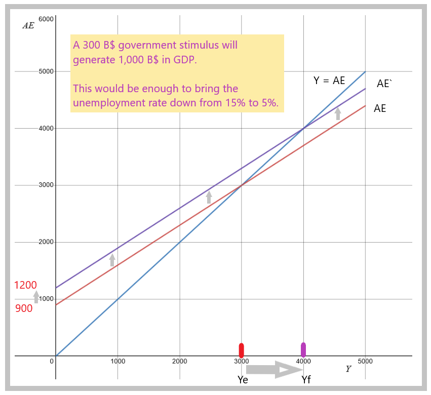
As you can see on the graph, a 300 B$ stimulus package was sufficient to solve a 1,000 billion dollar gap in output. This is because the money does not sit, people spend it. And since they save at a 30 percent rate, we can assume they spend 70 percent of the stimulus money. That means the money will cycle 3.33 times in the economy, so that 300 B$ of stimulus is multiplied into 1,000 B$ of output. We will explain this in more detail.
-
Limitations
There are important limitations to this model. First of all, its aim is very limited: to depict the effect of a drop in aggregate expenditure on overall production levels, and employment. The model does not factor in any kind of explanation of economic growth in the long-run. Austrian economists, such as Friedrich von Hayek, have argued it does not factor in the role of the private sector, which can invent new products, open new opportunities to invest.
Second, it does not factor in the role of market prices, or inflation. When prices drop during a recession, people can buy more stuff with the same income. The model assumes constant prices.
Third, the model assumes rich people have the same savings level as poor people. As income rises, the savings rate should increase. But the model assumes a constant level of savings. This is not issue of arithmetic, since the average is always based on the aggregate measure. It rather needs to be taken into consideration when choosing the ways that fiscal policy will be conducted.
Fourth, the model makes no account of a “supply-shock”, for example if resources are limited by a strike, war, or a natural disaster. The model was created to show how government intervention can multiply GDP when the economy is under-producing. It does not deal with any suppliers, or the problems they may have in meeting aggregate demand. In the wake of the COVID-19 pandemic, the world economy was subject to a major supply-side shock and this model is not of much use for that.
Fifth, the model is obsessed with the savings rate, which determines consumer spending. Keynesians are thus encouraging people to save less, during a recession, shifting focus away from productive investment in risky ventures that increase productivity, and towards focusing only on increasing consumption. More houses and more cars will not help build a more productive, and prosperous, economy in the future. More of the same is expansionary, but it is not economic development.
-
Solving for Equilibrium
AE is given by expenditures C, I, G, X-M.
AE = C+ I + G + X-M
AE also includes induced expenditures which are a function of aggregate income: MPC*Income.
AE = (Ca + Ci) + I + G + X-M
if, Ci = MPC*Income
then, AE = Ca + I + G + X-M + MPC*Income
At Equilibrium, AEe = Incomee
therefore, Incomee = Ca + I + G + X-M + MPC*Incomee
Incomee - MPC*Incomee = Ca + I + G + X-M
(1 - MPC)*Incomee = Ca + I + G + X-M
Incomee = (Ca + I + G + X-M) / (1 - MPC)
If the autonomous expenditure levels and MPC are known, then we can solve for the equilibrium income level.
Example:
if, Autonomous Expenditure = 1,200 B$, and MPC = 0,7,
then, AEe = Incomee = 1,200 B$ / 0.3 = 4,000 B$
-
The Government Multiplier
Keynes is arguing that the government does not need to fill the entire production gap with fresh spending. Because money circulates several times in the economy, a relatively small injection of funds can fill the gap. This is quite interesting for policymakers because fresh money does not come cheap.
The government multiplier (GM) is a ratio of how many times the extra government money can turn into output.
GM = (New equilibrium Income – Previous equilibrium Income) / Government Injection
Since the new production level depends on the MPC, the multiplier depends on how much people save, vs. consume, their extra income. This equation is the inverse of the MPS, which is equal to 1-MPC.
In other words: the autonomous spending, or any addition to autonomous spending, should be considered as the FIRST ROUND of spending in an economy. When someone’s spending becomes someone else’s income, then there is a SECOND ROUND of spending. And so on...
The number of rounds depends on the MPC, that is, the share of earned income that will be spent on product. The multiplier basically tells you the number of rounds. If MPC is 0.8, you will have 5 rounds of spending for each additional autonomous dollar. This means that a 20 B$ stimulus (extra G), will generate five times that amount in terms of GDP at the end of the year, or 100B$.
Here is the math:
GM = 1 / ( 1 - MPC )
The multiplier allows us to calculate the level of government intervention needed to fill in an output gap.
∆Y = ∆G * GM
Where ∆Y = Output gap, or the difference between Potential Real GDP and actual levels of Real GDP.
For example, if MPC = 0.8, then GM = 5. In this case, an output gap of 100 B$ would be solved by an added 20 B$.
∆Y = ∆G * GM
100 B$ = ∆G * 5
∆G = 100 B$ / 5 = 20 B$
In another example, using the data from the previous graphs, if MPC = 0.7, then GM = 3.33. In this case, an output gap of 1,000 B$ would be solved by an added 300 B$.
∆Y = ∆G * GM
1,000 B$ = ∆G * 3.33
∆G = 1,000 B$ / 3.33 = 300 B$
-
Principles
Positive:
There is an equilibrium level of production that matches aggregate income and aggregate spending.
It is possible to see a stable equilibrium level of production associated to a large and stable output gap, and associated surplus of labour (unemployment).
Normative:
Government should intervene if the output gap, and its associated labour surplus is too large.
Wrap-Up
A macroeconomic theory is a set of assumptions and logical deductions that help us predict outcomes in the economy.
The AE model is based on Keynes’ description of Aggregate Expenditure.
Positive shifts of AE create jobs, negative shifts AE create unemployment. In this case, government should increase expenditures to compensate and bring production levels back to equilibrium.
Cheat Sheet with Memory Helper
Aggregate Expenditure:
A curve that represents autonomous levels of spending, and induced spending which rises with income.
45 degree curve:
A curve that represents all levels of production for which Say's Law is respected, that spending equals income.
Government Multiplier:
A calculation of the multiplier effect of added government spending on GDP, based on the marginal propensity to consume.
References and Further Reading
Hicks, J. R. (1937). Mr. Keynes and the "Classics"; A Suggested Interpretation. Econometrica. Vol. 5, No. 2, pp. 147-159 (13 pages). https://www.jstor.org/stable/1907242
James, E., Wellman, S. J. & Aberra, W. (2010). Macroeconomics, 2nd ed. Pearson Canada. Chapter 9.
Keynes, J. M. (1936). The General Theory of Employment, Interest and Money. London: Palgrave Macmillan.
Samuelson, P. A. & Nordhaus, W. D. (2004). Economics, 18th edition. McGraw-Hill/Irwin. Originally published in 1948.
Say, J.-B. (1803). Traité d'économie politique.
Stiglitz, J. E. & Walsh, C. E. (2006). Economics, 4th Edition. New York City: W.W. Norton.
Thomas, A. M. (2021). Macroeconomics, An Introduction. Cambridge University Press.