Long-Run Consensus Macroeconomic Theory

Why Should I Care?

Comparing actual production levels to the full potential of our economy is useful to understand whether or not the government should intervene to create jobs, or to stem inflation.

This Lecture Has 5 Parts

• What is the Long-Run?
• Long-Run AD
• Long-Run AS
• Explaining Recessions
• Explaining Over-Heating

What is a Long-Run Macroeconomic Theory?

We will add the potential output to the AD-AS model. This helps to benchmark the economy’s actual production levels, and guide government intervention.

Video - Khan Academy LRAS

• What is the Long-Run?

The “run” refers to a theoretical framework where variables may or may not be changed (James, 2011: 224). This has nothing to do with short-term, or long-term, concepts, which refer to a time frame.

In the short-run, most variables are fixed, such as physical capital (buildings, machines), and land (minerals, energy). One variable is not fixed: labour. The only way to increase production is to hire more workers, or have them work more hours. When you decrease production, labour gets fired, but not the machines.

In the long-run, none of the variables are fixed. The economy’s resources are optimally allocated in order to maximize production, without over-using them. When you increase production, you increase all the factors of production, including labour, and capital.

Definitions

Short-run
A modelling format where some variables are fixed, and others may vary. Usually, physical capital is fixed, while labour costs are variable.

Long-run
A modelling format where all variables may vary, including physical capital.

Short-term
A time-frame that is short, such as 6 months, or less than 2 years.

Long-term
A time-frame that is long, such as more than 20 years.

• Long-Run AD

In the long-run, there is no reason to believe that the level of prices would not affect people’s real consumption. Inflation will always reduce purchasing power. Therefore, the aggregate demand curve keeps its’ position and shape as a downward sloping curve. Long-run AD is the same curve as short-run AD.

Also, the AD curve would shift the same way, whether the exogenous shift is a long-run change, or a short-run change. For example, if long-run expectations improve, you shift the AD to the right. If short-run expectations improve, the curve also shifts to the right.

• Long-Run AS

SR-AS
An upward sloping curve that represents the economy's capacity to produce in the short-run, where increasing output is associated to increasing costs of production.

LR-AS
A vertical curve that represents the economy's capacity to produce in the long-run, which is not a function of prices, but a function of available resources.

In the long-run, the supply scenario is different than for demand. On the supply side, we have to have two curves. The level of prices affects the output of the economy, but it does not affect the productive capacity of the economy. For this reason, the short-run aggregate supply curve is upward sloping, and the long-run aggregate supply curve is vertical. This is because the long-run AS curve represents a situation of full employment when production is at full capacity. In this situation, output is fixed at the optimal level, no matter what the price level is. This concept is the same idea as we saw in the Production Possibility Curve.

Graph - SR-AS, LR-AS and AD

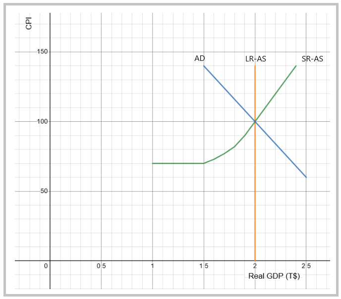
In this graph, the three curves meet and form an equilibrium which is stable in both the short-run, and the long-run, where Real GDP is 2 T$, and the price level is CPI = 100.

Long-run AS (LR-AS) is useful in showing the difference between the actual level of production in the economy and its capacity.

Play with the Graphs

Use the following link to have access to a Desmos graph of the AD-AS model. Geek out and play around with the curves, you can make them appear, and disappear. You can change the slopes and calculate output gaps.

https://www.desmos.com/calculator/pr6plljdjb

Factors that affect Short-run Aggregate Supply (SR-AS) will also shift the LR-AS curve. However, the difference is that these shifts need to be permanent in nature. For example, an increase in population, radical technological change, or an increase in the Participation Rate (Women entering the Labour Force), will shift both SR-AS, and LR-AS to the right.

For example, economists usually posit that an increase in taxes which is perceived as permanent by the population will have a negative impact on LR-AS.

Canadian economists feel that the LR-AS curve is constantly shifting to the right because of constant innovation, and population growth. This makes the “sweet spot” a moving target. Economic growth, as opposed to expansion during the business cycle, is thus a long-run phenomenon. In this way, LR-AS is another way of expressing ideas in the production possibility frontier model. When technology and capacity increase, so does the productive potential of an economy. Given the importance of environmental issues, growth has become a critical issue. It may be possible to keep growing the economy in monetary terms, but not in physical terms, since the earth's resources are becoming depleted by over-population and over-consumption. However this possibility has not been verified empirically yet.

Note that the SR-AS curve can “outproduce” the LR-AS potential. This is because in the short-run, producers can over-use their resources, by asking workers to work overtime, or by excessively using machines. This is not deemed “optimal” in the long-run, and can be dubbed as “stretching the elastic.”

Note: the Long-Run AS curve is a very theoretical position, and represents a “benchmark”, to be kept in mind, in the background.

Long-Run Model

• Definitions
  1. Long-Run: no variables are fixed.
  2. Potential output is a function of the quantity and quality of

• Assumptions
  1. It is possible to calculate potential output.
  2. None of the resources are idle.

• Hypotheses
  1. Over-production is not sustainable in the long-run.

• Predictions
  1. Producing more than potential is inflationary.
  2. Producing less than potential is recessionary.

• Principles

Positive:
Aggregate supply increases are deflationary.
Aggregate demand increases are inflationary.
Insufficient aggregate demand creates a stable output gap and associated surplus of labour.

Normative:      
(Left-wing)
Government should use its borrowing power to stimulate the economy if there is a recessionary output gap.

(Right-wing)
Government should beware its interventions are usually inflationary in the short-run.
In the long-run, government intervention should focus on helping to increase productive capacity (physical capital, labour, land) and aggregate supply.

• Explaining Recessions

Economic output is represented as the equilibrium of AD and SR-AS. When output also equals long-run potential, the economy is at full-employment. This is what we call the “sweet spot”. However, when the short-run equilibrium is inferior to potential, we call this a recession.

During a recession, low demand across all markets will soften price levels. This however depends on how bad the recession is and how close to potential the economy was when the slowdown started. During a recession, factor markets, such as natural resources, physical capital, and labour, will see their demand levels decrease. We don't suppose any substitution effects in the short-run so we can say that these markets would be in a surplus market condition.

Graph - Government Intervention Attempts to Bring AD Back to Potential

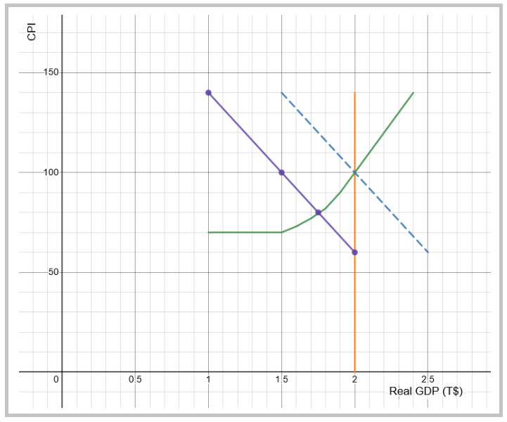
As you can see on the graph, the recession left a 250 B$ output gap, the CPI has dropped to 80, and you can imagine the unemployment rate has ballooned to double-digit territory. The Finance minister's team of economists has calculated that a 50 B$ stimulus program (using a multiplier of 5) would be enough to fill the 250 B$ output gap caused by the recession. How many subways, tramways and high-speed train projects could Ottawa afford with 50 B$ ?

• Explaining Over-Heating

During an expansion phase, increased demand generates more production and higher prices. When this creates paid work, the economy is doing its job. But when AD is expanding too much, past potential output, this added spending will be inflationary, creating shortages in resource and product markets. Too much spending can be caused by consumers, investors, governments, or foreign demand (exports).

Graph - An Over-Heating Economy

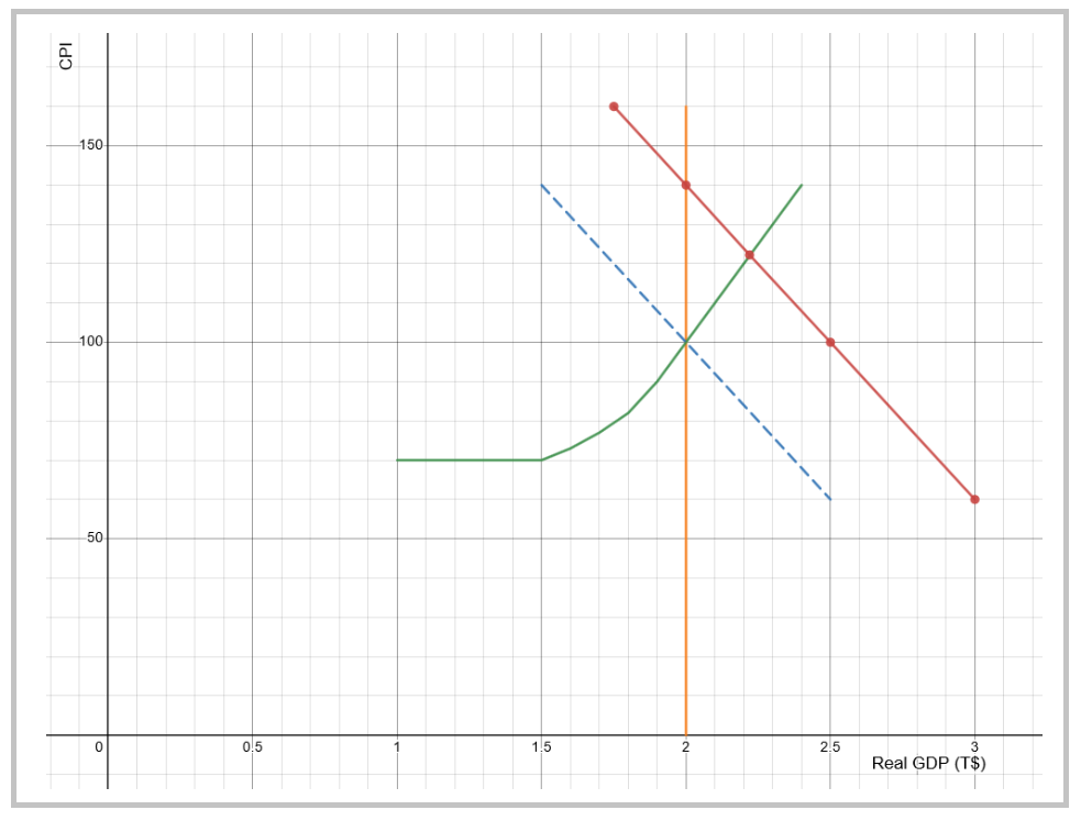
An over-heating economy is when GDP has grown larger than Potential GDP. In macro-economic terms, this is when the short-run equilibrium is producing a higher output than the long-run capacity. Remember that it is possible to out-produce LR-AS in the short-run, but it is a temporary position. The economy will be over-using resources and high prices across all industries will result from the over-heating of the proverbial hot-stove.

In this example,output is now at 2.22 T$ while CPI has increased to 122. You can imagine the unemployment rate is very low, and most probably at the level of full employment. Shortages on the labour market will not be visible using the unemployment rate, but using other metrics such as unfilled positions.

The output gap is a positive 220 B$. Government intervention would be to decrease government purchases, and increase taxes, by 44 B$. We obtained this figure by assuming a multiplier of 5. Price levels would come back to normal. In terms of business cycles, this policy would end the over-heating, but might spring the economy into a recession.

Wrap-Up

In the long-run, the economy is producing at optimal, full-potential output, at full-employment.

Having this benchmark helps to compare actual production levels to the desired level of production. If we are under-producing, we will have unemployment. If we produce too much, prices will rise too high.

In the short-run, keep in mind that suppliers can stretch the elastic and produce more than potential.

The long-run potential is constantly growing because of innovation and population growth. This makes the “sweet spot” a moving target.

Cheat Sheet with Memory Helper

Short-Run:
A theoretical framework where most variables are fixed, such as wages and capital.

Long-Run:
A theoretical framework where all variables are not fixed. LR-AS represents potential output when resources are not idle.

References and Further Reading

Blanchard, O. (2009). The State of Macro. Annual Review of Economics. Vol. 1, pp. 209-228 (20 pages)

Dornbusch, R., Fischer, S. and Startz, R. (2001). Macroeconomics, 8th edition. New York: Irwin/McGraw-Hill.

Jones, C. I. (2020). The End of Economic Growth? Unintended Consequences of a Declining Population. NBER Working Paper.