Market Disruption

Why Should I Care?

Markets are supposed to be stable and self-regulating. But social and natural events can disrupt markets and wreak havoc on regular peoples’ lives. Predicting how markets will react to outside factors can make you rich, or at least avoid becoming poor.

This Lecture Has 3 Parts

Shifts in Demand and Supply
New Equilibrium
Applications in VillageTown

What is a Market Disruption?

Markets are stable and self-regulating. Under an assumption of perfect competition, buyers and sellers react to changes in price, that’s obvious. That is the Free Market Mechanism, which sets equilibrium prices and output. Even in a monopoly, the market is in a stable of equilibrium.

But changes in nature like an earthquake, or social events like a labour strike, can disrupt an otherwise stable market. There will be a “new normal”, a new equilibrium. The supply and demand model enables us to predict the market outcome of such disruptions. The trick is to analyze changes to the demand and supply curves independently.

Shifts in Demand and Supply

The Marshallian model allows us to sort out the effects of a multitude of factors that can change the quantities of product on a market.

Essentially, the variables are sorted out where Qs, and Qd, are a function of several factors. Quantity is thus considered a Dependent variable. All other variables explain quantity, so they are considered Independent variables. In essence, its a clever model, because you actually have two dependent variables, which are very similar (Q_d and Q_s).

Q_d = f ( Price, Population, Income, Expectations, Tastes and Preferences, Prices of related goods )

Q_s = f ( Price, Number of producers, Prices of related goods, Technology, Expectations, Price of Inputs )

Both of these quantity variables will inter-act with each other, through the price variable. This is where the magic really lies. Both Q_d and Q_s are dependent on Price, but react differently to Price, which allows us to establish an equilibrium, or not.

Since the Price of a good influences both Q_d, and Q_s, the Price variable was chosen to be on the graph at all times (vertical axis). Q_d and Q_s are also on the graph, simultaneously on the same axis (horizontal). Price and Quantity are therefore considered ENDOGENOUS variables. Any change in Price is always included on both the Supply curve, and the Demand curve. The market graph has already taken this into account.

All other variables are EXOGENOUS. Their effect is not already factored into the Demand and Supply curves. Their effect will SHIFT either curve. An exogenous shift will bring about an unbalance in the market forces, a market condition of shortage, or surplus. This will generate a change in price, which will move the Qs and Qd along the new curves.

An example: new robots will increase production without increasing costs. More robots will increase the supply of automobiles.

Table - Sorting out market variables

Variable	Moves Curve	Function	Role in model
Qs	No	Dependent	Endogenous
Qd	No	Dependent	Endogenous
Price	No	Independent	Endogenous
Population	Demand	Independent	Exogenous
Income	Demand	Independent	Exogenous
Expectations	Demand	Independent	Exogenous
Tastes and Preferences	Demand	Independent	Exogenous
Prices of related goods	Demand	Independent	Exogenous
Number of producers	Supply	Independent	Exogenous
Prices of related goods	Supply	Independent	Exogenous
Technology	Supply	Independent	Exogenous
Expectations	Supply	Independent	Exogenous
Price of Inputs	Supply	Independent	Exogenous

Economists can predict how the market will react to these shifts because they suppose certain behaviours and relationships ahead of time. The factors mentioned will shift the whole curve, whether demand or supply.

The curve will shift left if demand (or supply) decreases, or right if it increases. (The curve does not shift up or down, it shifts horizontally along the quantity axis keeping prices constant.)

Why does the curve shift?

These outside factors are exogenous variables. They are “game-changers” that were not taken in consideration when building the theory, which focuses on prices and quantities. Price is an endogenous variable, which means it is included on the graph. This is why changes in price are already accounted for in the shape of the demand curve. In plain English, for the same price, people’s demand has completely changed for the product. You could say they love the product more, or less, for the same price. Because the “love” has changed, there has to be a new curve to depict the new level of demand.

Market Changes and the Reaction of Buyers

Market Change	Buyer’s Reaction	On graph
A - Price increases	Love it the same, but buy less	Qd slides to the left
B - Price decreases	Love it the same, but buy more	Qd slides to the right
C - External factor increases Demand	Love it more, Buy more at same price	Qd jumps right
D - External factor decreases Demand	Love it less, Buy less at same price	Qd jumps left

~~Scenario~~Scenarios

Here are some market values for different products. Qe represents an equilibrium market production level where Qd = Qs. For each market, a demand-side shock triggers a disruption.

Product	Price ($)	Qe / mth	Shock	New Qd	Price change	New Qe
Shoes	600	100	Out of fashion	50	Down	50-100
Ice cream	5	250	New immigrants	300	Up	250-300
Internet Access	45	3,000	New movies on Netflix	4,000	Up	3,000-4,000
iPhone 11	700	400	iPhone 12 released	350	Down	350-400

The supply and demand framework allows us to identify where the market will be going. But it's not possible, at this level of analysis, to be really precise about the final Quantity and Price the market will settle on. For example, if a certain model of shoes go out of fashion, of course the Quantity demanded would decrease, and those shoes will be on sale. This is pretty predictable. Where the model adds value to our analysis, is to keep in mind that as the price goes down, a few more people will buy those shoes. The quantity decrease, in the end, will not be as drastic as a simple analysis would predict.

Keep in mind that when a market is disrupted, economists have to make assumptions about the slope of each curve, in order to find a new equilibrium. If the demand and/or supply curves were steeper, or flatter, the final equilibrium won't end up at the same place.

Market Changes and the Reaction of Sellers

Market Change	Seller’s Reaction	On graph
A - Price increases	Encouraged to produce more	Qs slides to the right
B - Price decreases	Discouraged, will produce less	Qs slides to the left
C - External factor increases Supply	Capacity to produce more, for the same unit price	Qs jumps right
D - External factor decreases Supply	Capacity to produce less, for the same unit price	Qs jumps right

New Equilibrium

The shifts in Demand and Supply create disruptions on the market for any good or service. But before you shift any curves, make sure you understand what to do, and the proper sequence of the model.

Supply and Demand Algorithm

The first step is to identify what's going to move on the graph.

Who is affected first and foremost?
> Producers: Supply curve
> Buyers: Demand curve

Is this a price change?
Yes > Price shock: Quantity will slide
No > External shock: Curve will shift

Which direction?
> More quantity: Right
> Less quantity: Left

Let’s say a sunny heat wave is increasing demand for sunglasses.
1- This will affect buyers, so it affects the demand curve (DD).
2- This is an exogenous shock, so the Demand curve will shift.
3- Buyers will buy more, at all prices, so DD will shift right.

The second step is to identify the market condition that will move the price, and generate adaptation.

Is it a shortage or a surplus?
> Shortage Price increases
> Surplus Price decreases

Adaptation
> Price increases Qd slides left, Qs slides right
> Price decreases Qd slides right, Qs slides left

Let’s say a sunny heat wave is increasing demand for sunglasses.
1- The shift in demand creates a shortage, which increases prices. New Qd slides left, Qs slides right, to new equilibrium.
2- End result, higher prices, higher quantities.

Applications in VillageTown

The ladies in VillageTown are operating as a competitive oligopoly, so we can draw both demand, and supply curves.

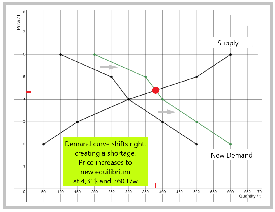
Increased Demand

In this first scenario, there is an influx of new population in the village, which will increase demand for ice-cream. Let's assume Qd increases by 100 L/w for each price point.

Table - Increased Demand

Price ($/L)	Qs (L/w)	Qd (L/w)	New Qd (L/w)
6	600	100	200
5	500	250	350
4	300	300	400
3	150	400	500
2	50	500	600

Graph - Increased Demand

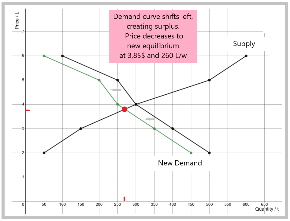
Decreased Demand

In this second scenario, there is a drastic change in people's preferences. VillageTowners are going vegan, which will decrease demand for ice-cream. Let's assume Qd decreases by 50 L/w for each price point.

Table - Decreased Demand

Price ($/L)	Qs (L/w)	Qd (L/w)	New Qd (L/w)
6	600	100	50
5	500	250	200
4	300	300	250
3	150	400	350
2	50	500	450

Graph - Decreased Demand

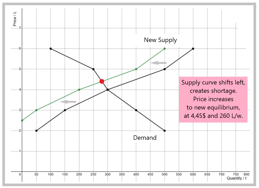
Decreased Supply

In this scenario, there is an increase in input costs in the village, which will increase cost of production for ice-cream. Let's assume Qs decreases by 100 L/w for each price point.

Table - Decreased Supply

Price ($/L)	Qs (L/w)	New Qs (L/w)	Qd (L/w)
6	600	500	100
5	500	400	250
4	300	200	300
3	150	50	400
2	50	-	500

Graph - Decreased Supply

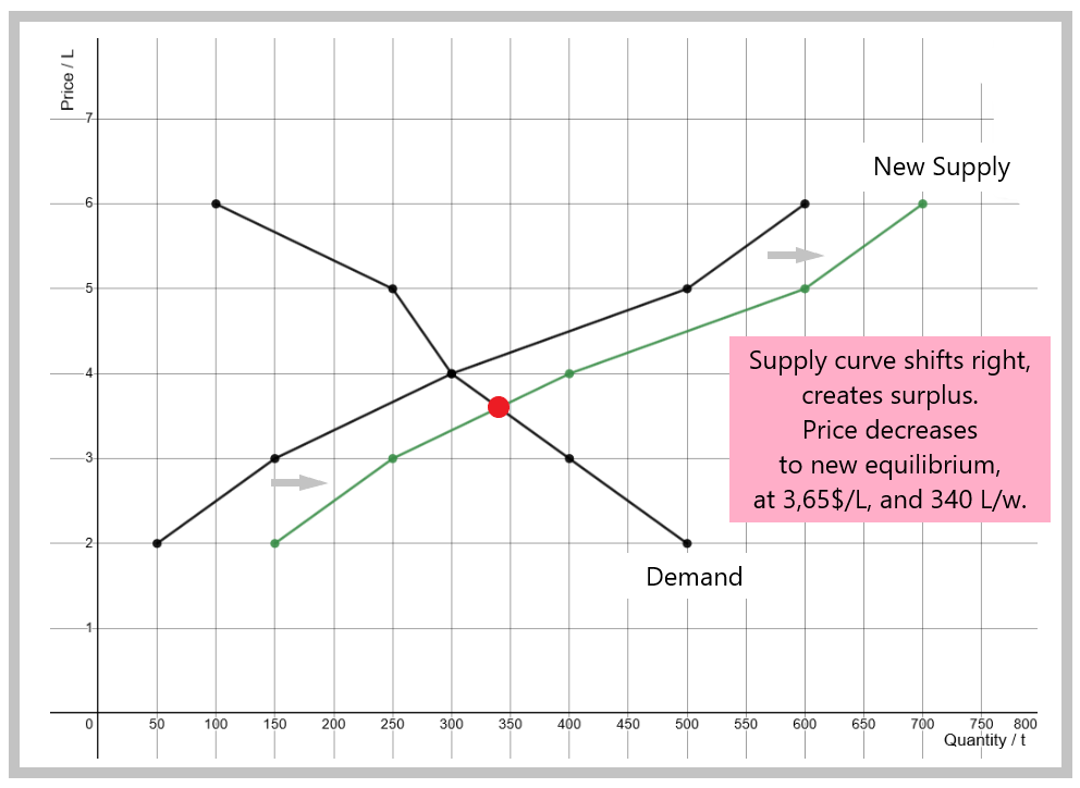
Increased Supply

In this scenario, there is an increase in capacity, due to the invention of new robots. This will decrease costs of production for ice-cream. Let's assume Qs increases by 100 L/w for each price point.

Table - Increased Supply

Price ($/L)	Qs (L/w)	New Qs (L/w)	Qd (L/w)
6	600	700	100
5	500	600	250
4	300	400	300
3	150	250	400
2	50	150	500

Graph - Increased Supply

Green Policy

Many economists believe that you can use the market mechanism, the Marshallian Supply and Demand model, to reduce pollution. The trick is to include the social cost of pollution into the final price of the product. By taxing BADS, you can swiftly impact meaningful change without sending anyone to jail, or having the government make critical allocation decisions. The market can solve the problem.

How this works is simple. A tax is a supply factor. An increase in taxes will shift the supply curve to the left. As markets adapt, part of the increased tax will turn into a higher price for consumers, and part of the tax will decrease the quantity of sales of the BAD product.

Note that this type of policy works best when there are alternatives which are ready and waiting to be consumed. If you tax, without preparing an alternative product, the consumers will bear the brunt of the tax and there won’t be a reduction in quantity.

Climate Change Solution

Most economists agree that a tax on carbon is a fair and efficient solution to reducing GHG emissions. Rather than ask consumers to stop using their cars, implementing a tax on gasoline would have a direct impact on demand for gasoline, and for cars. It’s fair because those who are responsible for emitting GHG’s have to pay for it.

The capitalists and the industrialists will receive a clear signal that these products are doomed, and their efforts show be going towards GHG-free production. One would expect consumers, as well as producers, to look for alternatives (substitution effect).

Democracy Booster

It is obvious that many industries stand to lose millions and billions of dollars if carbon taxes were to be implemented. However, it is not economical to leave the situation as it is. Money never disappears. It would be invested in cleaner projects. This is not a lose-lose scenario. It is a win-win scenario.

Wrap-Up

Markets are stable, but society is not. An outside change will disrupt markets. But markets do stabilize, in theory, at a new equilibrium because of the market forces behind the theory of supply and demand.

This new combination of price-quantity will be stable. To find it, and predict it properly, shift the proper curve according to the relevant factors. Suppliers and demanders will meet once again at the new equilibrium combination of price and quantity.

Cheat Sheet

Price shock:
A change in price that affects the quantity demanded or supplied of a particular product.

External shock:
A social or natural event that deeply affects the supply or demand curve.

Demand shifters:
Income, Tastes and Preferences, Expectations, Demographics, Supply of Related Goods.

Supply shifters:
Number of producers, Change in technology, Demand for Related products, Expectations, Input costs.