Supply
Why Should I Care?
Producers come to the market with a completely different mindset than do buyers. Producers want more money for fewer products. How can they agree with buyers, who want more products for less money? Understanding the supply-side of the story helps us understand how markets work, because without producers, no one gets products.
This Lecture Has 5 Parts
- Law of Supply
- Perfect Competition Theory
- Supply and Quantity supplied
- Factors Affecting Supply
- Limitations
What is Supply?
When producers sell their final products, they are supplying the market with goods and services. Their ability to do so affects prices and quantities. This mostly has to do with how they manage their costs, and what technology they use.
In economics, the formal concept of “supply” refers to a set of possible, hypothetical, and technologically consistent transactions suppliers would be ready to accept on a market.
-
Law of Supply
Suppliers are attracted to markets with high prices. When the price on a market increases, this lures more producers to the industry, and increases quantities supplied. This is also true in the reverse situation. If prices decrease, suppliers will decrease their production or leave the market completely.
This is the Law of Supply.
All things equal, when price increases, quantities supplied increase as well, and vice-versa.
There are actually a few reasons why this assumption is useful in economics.
First, suppliers are sensitive to incentives. A high price is a strong incentive to produce more goods and services because it leads to a multiplication of potential income for the industry.
Second, suppliers are subject to opportunity costs. Producers can substitute their decisions between similar markets. If the price increases on one market, it increases the opportunity cost to not make that good or service, which serves as a further incentive to enter the market.
Third, suppliers are subject to production costs. As production grows, so do costs, so we should expect suppliers to ask for higher prices at higher production levels. Production costs act as an indicator of capacity. At a certain point, the suppliers cannot produce more and the production costs become infinitely high.
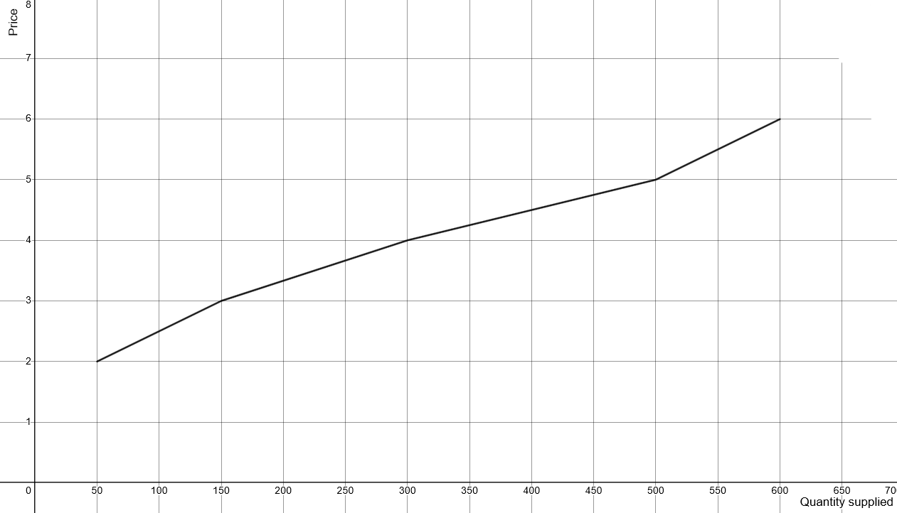
A supply curve represents this relationship. The curve includes the various quantities of a good or service that sellers are willing to produce at various price points, over a specific period of time. Supply represents a flow, not a stock, of goods. We measure output over time, such as Quantity supplied per week. Quantities can be measured by unit, such as the number of chairs produced per week, or by dollar value, such as total sales per week.
Why? Because we wish to explain production that is supplied to market, not production that is idle. Stocks of goods are not necessarily consumed; they are often sitting in a warehouse. Goods are flowing because they are sold and consumed over time.
Supply: Quantity is a positive function of prices Qs = f (P)
If Price INCREASES, then Quantity INCREASES.
If Price DECREASES, then Quantity DECREASES.
-
Perfect Competition Theory
To chart a supply curve, we have to assume a very critical and controversial idea: perfect competition.
In economics, the idea of a competitive group of suppliers is characterized by the supply curve. But the existence of a supply curve depends on the assumption of perfect competition. That is: there are enough producers to keep prices as low as possible. Also, the product is not unique and can be easily copied and substituted.
In this scenario, economists assume that no one supplier has an “edge” in the market to draw clients, other than prices. Every one’s product is the same quality, the customer service is the same, the locations are the same, etc.
Theory of Perfect Competition
- Definitions
- Producers are called suppliers.
- Suppliers must sell at a price that covers production costs.
- The market is open (arbiter sets single price).
- Assumptions
- Suppliers are numerous and very competitive.
- Suppliers cannot “Cherry-Pick” price-quantity combinations.
- The product is a homogeneous commodity (not differentiated)
- Hypotheses
- Suppliers require higher prices to increase production
- Predictions
- The intersect of the demand and supply curves sets the open-market price
- Any producer who does not conform to market price will not cover production costs because of lower sales or excessive costs.
- The equilibrium market price, and market quantity, is stable.
-
Supply and Quantity supplied
Economists distinguish between the supply curve and levels of production called Quantity supplied (Qs). It's important in terms of modelling because we are going to use the framework to predict the effect of outside shocks on the behaviour of an industry. The interaction between buyers and sellers needs to be isolated, so we need to be specific.
If there was a shift in market price, then suppliers would increase their output, which means there would be a slide on the supply curve. The curve itself does not shift. It only shifts if there is an exogenous shock, which we will discuss in the next section.
Let's look at the situation in VillageTown. Grandma Jones is confronted to some unrelenting competition from her bridge friends Grandma Mimi, Mrs. Cupcake and Mama Roberta. Together, they make up a perfectly competitive ice cream industry. Grandma Jones is no longer the only game in town!
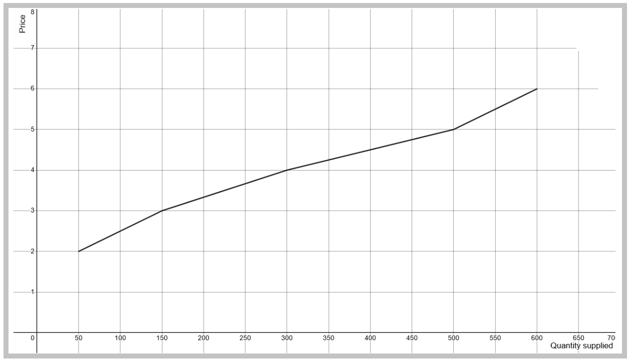
Table - Supply Schedule of Ice-Cream in VillageTown
| Situation | Price ($/L) | Quantity supplied (L/w) | Potential sales ($/w) |
| A | $ 6 | 600 |
$ 3,600 |
| B | $ 5 | 500 |
$ 2,500 |
| C | $ 4 | 300 |
$ 1,200 |
| D | $ 3 | 150 |
$ 450 |
| E | $ 2 | 50 |
$ 100 |
It is easy to see that the girls would love to produce at the highest possible price. If the market price is $2, the industry won’t want to make more than 50 tubs (1 Litre), because it takes a lot of time for the initial setup. It’s not worth spending hours preparing a batch, only for $100 sales, that need to be split across the four producers in some way or another. The ladies would rather use their time to play bridge together.
But if the price rises to 6 $/L, the old ladies will dump their mutual bridge game and make 600 tubs because they will make 36 times more money.
This is not necessarily going to be feasible because this all depends also on the level of demand. But the idea is important, Grandma Jones cannot control production. She can't stop anyone from being attracted to this market when prices are high.
There are lots of reasons why producers are attracted to high prices, but the main reason is the explosion of income. If you compare with a demand schedule, where total sales even out in between the extreme levels of prices, in the case of supply, the potential sales grow exponentially.
The graph below shows each Quantity supplied-Price combination, which makes up the Supply curve for Ice-Cream in VillageTown.
Graph - VillageTown Ice Cream Industry Supply Curve
-
Factors Affecting Supply
In this model, price and quantity are endogenous variables, which means they are on the graph, and they interact closely with each other. Any other factor is considered exogenous, which means it is not visible on the graph (in simple terms). We have seen the factors that affect demand, such as fashion, demographics, and income. The factors that affect supply have more to do with production capacities.
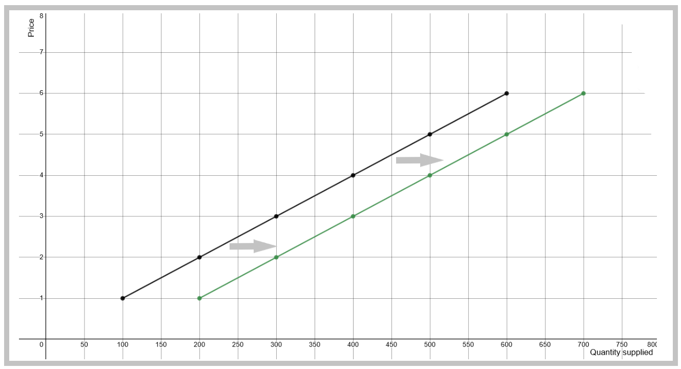
Always shift the curves along the quantity axis, that is left-right. The curves never shift up-down. An exogenous shift is assuming that prices are constant, which is why you are going to shift the curve horizontally.
Number of producers
If there is an increase in the number of producers, such as the arrival of a foreign company in your country, you can expect the supply curve to shift right, towards infinity. If there is a decrease in the number of producers, the curve shifts left towards zero.
Expectations
If there is an increase in expectations of future demand, the supply curve shifts right. A decrease in expectations will shift supply left.
Change in the price of inputs
If there is an increase in the price of raw materials, or any other input, you can expect the supply curve to shift left, towards zero on the Quantity axis. If input prices decrease, capacity increases, and the curve will shift to the right.
Change in the availability of inputs
Extreme shortages make the price of inputs irrelevant. If there is a decrease in the availability of inputs, the supply curve will shift left.
Change in technology
Improvements in technology, especially new production processes, allow producers to make more output, with fewer inputs. This can graphed with a shift of the supply curve to the right.
Change in the regulatory environment
If a product is banned, or its production is limited, such as firearms, or toxic chemicals, producers will reduce output. The supply curve will shift to the left. If regulations are removed, then production increases. The supply curve shifts right.
Change in the fiscal environment
If the government increases taxes on producers, production costs increase. This will shift the supply curve to the left. Inversely, if taxes are culled, production costs decrease, and the curve should shift to the right.
Graph - Increased Supply
-
Limitations
The Supply Curve model has an obvious limitation: it supposes perfect competition which can rarely be observed in real life. The first reason for this is that the model only applies to commodities, with no issues of quality or differentiation. Companies usually want out of this kind of cut-throat price-only-competition market. They will either differentiate their product to establish some kind of “niche” and reduce competition. Or, if their product is a true commodity, companies will spend – often obscene amounts – of money on advertising to increase customer loyalty.
At the same time, the industry will most probably consolidate the market into an oligopoly so that the meagre profit margins benefit to fewer companies. If the oligopoly colludes, profits increase through price-fixing.
Second, the model supposes perfect competition at all market sizes. However, we know competition grows with more production. Some markets are just too small for high levels of competition.
Third, the model makes no provision for economies of scale due to division of labour, transportation costs, and technology use. Often times, as production grows, costs actually go down. This is why many suppliers give discounts on bulk orders. There is a limit to this, and eventually costs rise.
Fourth, the curve might not be continuous in real-life, and it might not be a clean straight line. This is due to variable technology across producers. Some companies use brand-new machines which are very productive, and others use legacy systems that cost more to operate. Drawing a perfectly smooth line may not depict the actual situation of a particular industry.
Fourth, there is a simple gap in logic as to who sets the “market price” in the first place, if each supplier cannot set prices themselves. This gap is filled by the use of an arbiter, who matches the price preferences of demanders and suppliers, and imposes a single market price to all. This makes sense, but “arbitered” markets are very rare in real life.
Wrap-Up
The supply curve represents what producers are willing to make, for different price points. It is upward sloping because higher prices attract more producers, and help to cover increased costs.
The curve exists only under the assumptions of perfect competition, and applies only to commodities.
Cheat Sheet
Supply:
Combinations of quantities and prices of goods and services that suppliers are willing to produce.
Equilibrium:
A steady-state combination of price and quantity where demand equals supply.
Perfect Competition:
A theory that states that producers cannot influence the price or quantity of products, which are set by the open-market.
Commodity:
A good that is not different from a competitor’s product. Examples: gas, apples, iron ore, lumber.
References and Further Reading
Hill, R. & Myatt, T. (2010). The Economics Anti-Textbook. A Critical Thinker’s Guide to Micro-Economics. Halifax: Fernwood Publishing.
Stiglitz, J. E., & Walsh, C. E. (2006). Economics, 4th edition. New York: W. W. Norton & Co.


