Consensus Macroeconomic Theory

Why Should I Care?

Politicians spend your money. You might want to understand what their arguments are for increasing expenditures or changing tax rates. Hint: most of their arguments come from macroeconomic theory. This is the most used macroeconomic model, which bridges supply-side issues with Keynesian demand-side issues.

This Lecture Has 4 Parts

• Aggregate Demand
• Aggregate Supply
• Equilibrium
• Simulating Shocks to Predict GDP and CPI

What is Consensus Macroeconomic Theory?

There are dozens of macroeconomic theories, most based on deductive logic. Neither of them are perfect. However, these “models”, simpler representations of complex systems, can be useful to understand and predict the consequences of changes in investments, consumer spending, government expenditures, or even money supply.

The model we see now is called Aggregate Demand and Aggregate Supply (AD-AS). It is a consensus representation of the economy that tries to enable both Keynesian and Classical views of macroeconomic behaviors.

Keep in mind that we are building this model with a few assumptions which are listed later. This model is not the most sophisticated of its kind and is used for mostly pedagogical reasons. More advanced macro-economists use other types of models such as Dynamic General-Equilibrium Models (DGEM).

The basic assumption behind this model is that business cycles don't just happen regularly, they are treated as specific shocks. The model can then predict how a laissez-faire economy would react to the shock, usually by generating a production gap with potential GDP. Finally, policy makers can decide and plan a policy to help the economy move back to its potential output.

We are presenting a version of AD-AS with a price index (ex: CPI) as the vertical axis variable, and not the rate of inflation (percent change of CPI), which you would see in more advanced texts. This is done to simplify the basic understanding of the model's ideas.

We are also using Real GDP as the main output variable. This is especially important since the reason this model exists is to incorporate the effects of inflation into macro-economic policy. In a zero-inflation world, you can use the Keynesian Cross macroeconomic model.

• Aggregate Demand

This concept relates to how people act as a collective, a group, of spenders. Aggregate Demand (AD) was invented by Keynes.

AD = C + I + G + ( X – M )

The AD curve is not the sum of all the demand curves of the economy. It has the same shape as a regular demand curve. But not for the same reason. AD is based on aggregate, collective behavior. We suppose that people don’t change their behavior because of the inflation level. They don’t increase their spending when prices are low. The spending level is thought to be planned in advance, and constant.

The first reason that aggregate demand shrinks in high-price environments is that the planned level of spending equates to less product when prices are inflated. This is the wealth effect.

The second reason is that high prices force banks to increase interest rates, and this makes loans more expensive. This will translate to a decrease in the demand for loans, such as home mortgages and car loans, which decreases the demand for those products. This is the interest-rate effect.

The third reason is that local prices will affect the flow of trade. In a local high-price environment, exports will drop, and imports will rise. This equates to less product demanded. This is the trade effect.

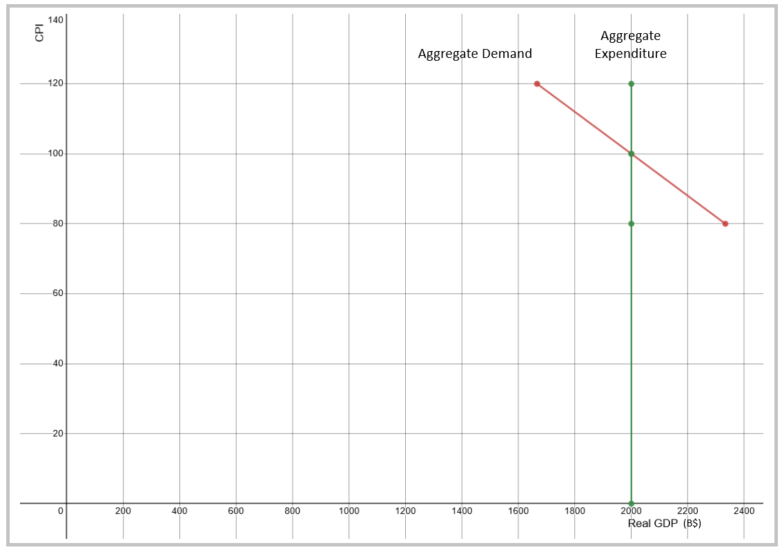
The following table shows the difference between Aggregate Expenditure (AE) which is framed in nominal dollars, and Aggregate Demand (AD) which is expressed in real dollars. Let's say the economy is at a base-level of inflation, where CPI is 100. Aggregate expenditure comes in at 2 trillion dollars, and consumers obtain 2 trillion dollars of product.

If inflation increases, and CPI jumps to 110, planned expenditures don't change. People still spend 2 trillion dollars in stores, who will declare 2 trillion dollars of income. But people are getting less product. In real terms, they are getting the equivalent of 1.8 trillion dollars worth (if prices were at CPI = 100). Spending has not changed, but real demand has decreased.

If inflation decreases, and CPI dives to 90, planned expenditures don't change. People still spend 2 trillion dollars in stores, who will declare 2 trillion dollars of income. But people are getting more product. In real terms, they are getting the equivalent of 2.2 trillion dollars worth (if prices were at CPI = 90).

Table - Planned Aggregate Expenditure vs. Planned Aggregate Demand

Price Level	Nominal Planned Aggregate Expenditures (Billions CA$)	Real Planned Aggregate Demand (Billions CA$)
Index base 100	AE (Nominal $)	AD (Real $)
120	2,000	1,666
110	2,000	1,818
100	2,000	2,000
90	2,000	2,167
80	2,000	2,333

As you can guess by now, the AD-AS model uses the concept of AD, not AE, in its graphs. High prices mean consumers purchase less product for their money. Low prices mean consumers purchase more for their money. The AD curve is therefore downward sloping when CPI is scaled on the vertical axis. Real output is scaled on the horizontal axis.

Graph - Planned Aggregate Expenditure vs. Planned Aggregate Demand

• Aggregate Supply

This concept relates to our collective capacity to produce. Resources are the key to understanding AS. An economy’s capacity to produce is a function of the quantity and the quality of its resources.

This can be written as the following phrase:

AS = f (K, N, L) + α

Where K is capital, N is natural resources, L is Labour, and α (alpha) represents the quality of the resources. Wages are held constant. In the short-run, producers can increase output, but in doing so, they use resources which are usually less productive, or create shortages in several markets.

A less productive resource could be an untrained worker hired because all the trained and experienced workers are already taken. This worker will not be paid more than others. But he will cost more to the producer because of his low productivity.

A shortage situation could increase the price of a resource such as raw materials or capital. If the economy is running at full speed, an increase in AS may create shortages in the market for steel, or tools. These higher prices for resources will increase the unit cost of production and increase the price of the final product.

The AS curve is upward sloping because more production increases production costs. Note that in this theory, suppliers are not reacting to high prices, they are creating them.

The idea that supply is expecting higher prices depends on how much utilization is being asked of the factories and the overall capacity of the economy. Well, according to Keynesians. The slope of the AS curve is actually an important bone of contention for economists, because it makes a big difference in how the simulation is going to predict what happens to output.

• Equilibrium

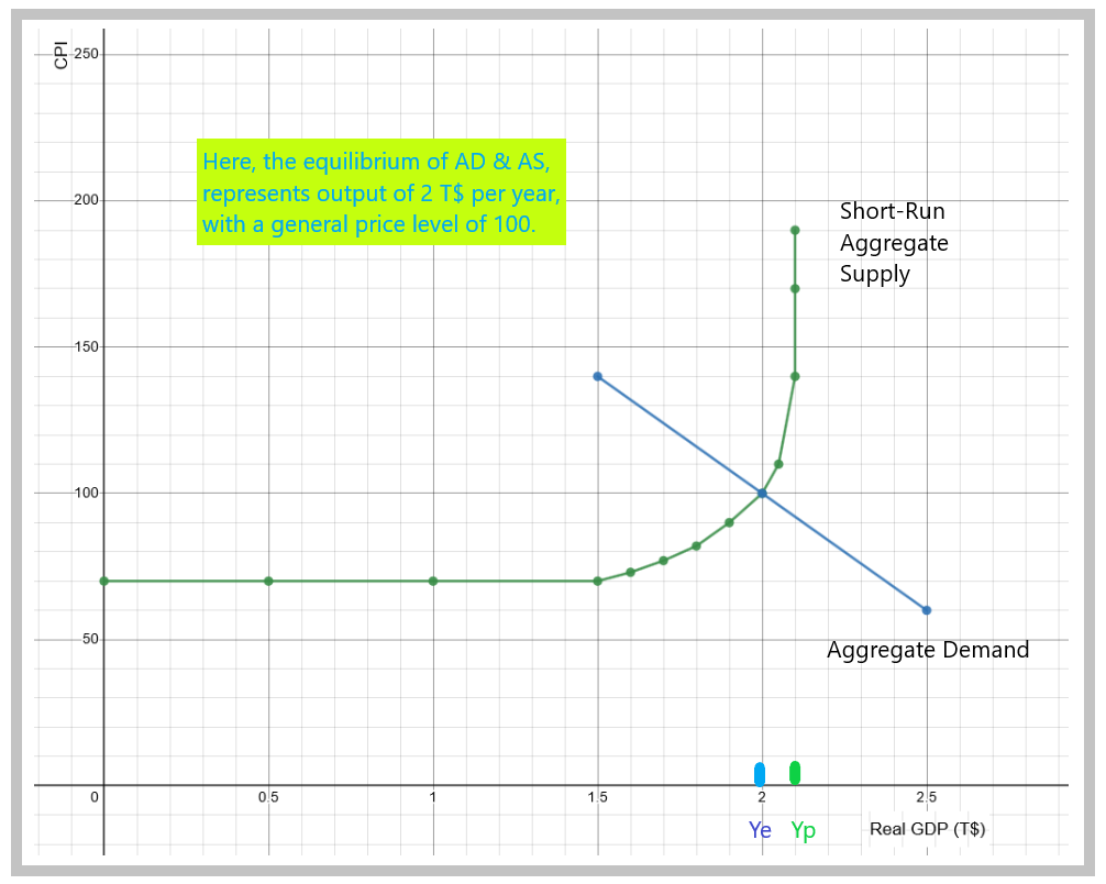
AD and AS meet at equilibrium. At this output level, prices are stable, and there are no market pressures to change the situation. If, however, the level of production were inferior to equilibrium, supply would be inferior to demand. This situation would not be stable because consumers would still be buying as much product, and inventories would be depleted. In turn, suppliers would increase production to replenish inventories. AS would shift back to equilibrium.

AS < AD, inventories shrink, production increases.

If the level of production were superior to equilibrium, supply would be superior to demand. Consumers would not be buying enough production. This situation would not be stable as production would halt as suppliers wait for inventories to be sold.

AD < AS, inventories grow, production halts.

Graph - Equilibrium Output at Base Price Level (B$)

AD-AS Model

• Definitions
  1. Aggregate Demand = C + I + G + (X - M)
  2. AD does not represent the sum of demand of all markets
  3. AD represents the collective behaviour of consumers
  4. AD represents planned expenditures for the near future
  5. Aggregate Supply = f(K, L, L) + α
  6. AS represents production capacity
     
     
• Assumptions
  1. Nominal aggregate spending is planned and constant.
  2. Wages are held constant.
  3. Changes to income streams flow directly to spending (AD), not to production capacity (AS).
  4. Increases in production increase marginal production costs.
  5. The equilibrium output level is set by the relationship between inventories and the price level.
  6. The model assumes no modern monetary policy. Left alone, a recessionary shock will be deflationary in the short-run.

• Hypotheses
  1. AD decreases in high price environments
  2. AS increases in high price environments
  3. Inflation is a result of production levels

• Predictions
  1. Increases in AD will increase output and prices.
  2. Increases in AS will increase output but decrease prices.
  3. Actual level of production must equal both AD and AS, if not, inventory adjustments will clear markets.

• Simulating Shocks to Predict GDP and CPI

The main objective of the model is to allow economists to predict changes in GDP, and related changes in employment and inflation levels, when there is a significant shock to the system. Previous models, such as the Keynesian AE model, do not include inflation levels. With the AD-AS model, you can predict the effect of a government stimulus package on both output (GDP) and price inflation (CPI).

The model does not really explain why and how recessions happen. But it does help to predict them, and how the macroeconomic aggregates react to shocks that are exogenous to the model. Since output and inflation are endogenous variables in the model (they are on the graph), any other variable is considered exogenous, and will affect the model by shifting one of the curves, either AD or AS.

So, what is an exogenous shock?

It is a significant change in any variable that could have an effect on either the aggregate demand, or the aggregate supply functions. Most of these shifters are social, political, and economic phenomena. On the demand side, changes in population, disposable income, expectations, foreign demand (exports), or government intervention can shift the AD curve.

On the supply side, changes in costs of labour and resources, quantities of labour and resources, or the quality of labour and resources (technology), can shift the AS curve.

Factors affecting AD and AS

Factors affecting AD	Factors affecting AS
Population	Technology – Labour productivity
Disposable Income	Resource Endowment
Expectations	Labour Quantity
Foreign Demand	Physical Capital Quantity
Government Intervention	Cost of Labour
	Cost of Resources

The model works in a very similar way to the micro-economic model of market supply and demand. Once you identify the shock and the related curve, you must interpret if it will mean more economic activity, or less. Then, you shift the curve left (less) or right (more).

The model will adapt to the shock by finding a new equilibrium. The interesting thing here is that you now have a prediction of the associated level of prices to this new level of economic activity.

For example, if a country's population increases, you shift the AD curve right. This will generate a certain amount of growth in GDP, but will also come at the expense of higher prices. For this to hold, we assume that all other factors are held constant, including supply factors (All Else Being Equal, Ceteris Paribus).

Generally speaking, an increase in AD will be inflationary. And conversely, a decrease in AD will be deflationary.

On the supply side, if you shift the AS curve right, on the interpretation of an increase in new production technologies, such as AI and robotization, this will generate some growth in GDP, and given that demand factors remain constant (All Else Being Equal), the price level in the economy will decrease.

How AD and AS are affected by exogenous shocks

Curve	Change	Shift	GDP	CPI
AD	Increase	Right	Increase	Increase
AD	Decrease	Left	Decrease	Decrease
AS	Increase	Right	Increase	Decrease
AS	Decrease	Left	Decrease	Increase

You can use the Keynesian model to establish the equilibrium output, we assume this level is associated to a base price level (CPI = 100). On this graph, equilibrium is set at 2 trillion dollars. The model becomes useful if you model shifts to AD or AS, and simulate the effect on GDP and CPI. In a classical example, a recession creates unemployment.

Graph - A Recession

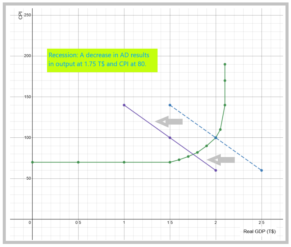
This graph shows a recession, which in Keynesian terms would be caused by a decrease in aggregate demand. Depending on where the AD curve sits on the AS curve, and the extent of the shock, the outcome would be a reduction of Real GDP, to 1.75 T$ and a decrease in CPI (to 80).

The government comes in with stimulus packages. If the output gap is 250 B$, the stimulus required would be 50 B$, using a multiplier of 5 (based on a 80% marginal propensity to consume).

If you are wondering about the multiplier effect, which is typical of Keynesian macroeconomics, you can apply the technique presented in the Keynesian model. In short, assuming a certain marginal propensity to consume (MPC), you can calculate the government multiplier (GM), and the appropriate stimulus (∆G), to fill an output gap (∆Y).

GM=1/(1-MPC)

∆G = ∆Y * (1-MPC)

You can't see the multiplier on the graph, but you can shift the AD curve to the right, by 250 B$. This will generate a new equilibrium. The model, and this is where the compromise with classical economists comes into play, takes inflation into account. The output level of 2.1 T$ would not be preferred, as it would see CPI jump to 140, which is wildly inflationary.

Hopefully, the economy would settle at 2 T$ and CPI of 100.

Graph - Stimulus Package to Fix the Recession

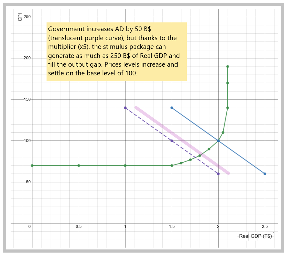
The graph shows what a stimulus package can do, whether it's fiscal or monetary in nature. In this case, the output gap was estimated at 250 B$. Assuming an overall multiplier of 5, the stimulus needed to fill the gap would be 50 B$. In the model, AD shifts to the right and the outcome is higher output, and higher prices. If the stimulus is too strong, the policy can be inflationary, as AD will shift too far to the right, and face a pent-up sloping AS curve.

The argument about the limiting effect of inflation on government intervention is quite strong. Debate over this issue is quite lively. For hard-core Keynesians, the model is especially useful in times of great recessions, or depressions, in which case the AS curve would be horizontal, and stimulus spending would be fully beneficial. For hard-core classicists, these situations are very rare and should not be used as a bench-mark for everyday macroeconomic policy. They believe in an upward sloping AS curve, which reduces the benefits of intervention.

Graph - Supply Shock Recession

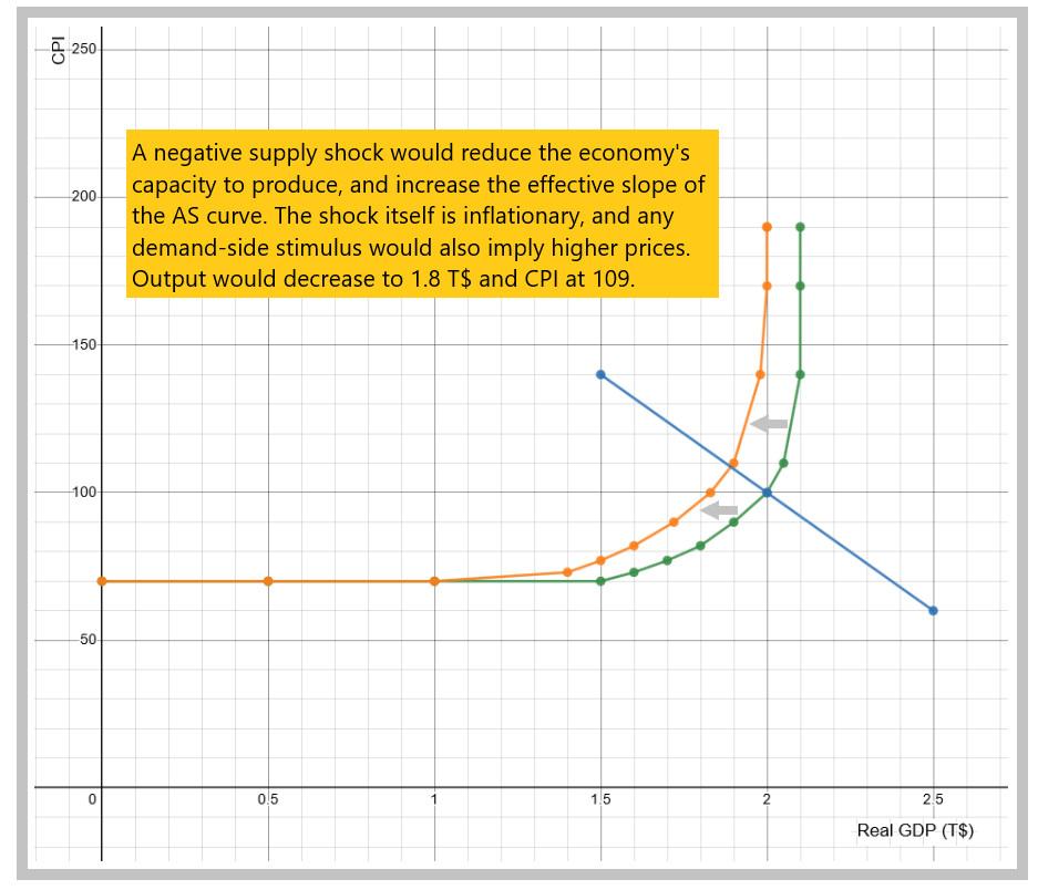
This graph shows the effect of a supply shock on the economy. A supply shock is an exogenous event, related to a variable which is not directly included in the model, such as a large labour strike, a sudden flux of migrants, a natural catastrophe, or a change in foreign demand for exports. If the shock is negative, it would reduce production capacity and shift the AS curve to the left. This is an explanation for a supply-side recession. This situation is not accounted for in purely Keynesian models.

Notice that in a supply-side recession, output decreases, but prices increase. In this case, CPI increased from 100 to 109. This is the kind of scenario that would explain what happened during and after the advent of the COVID-19 pandemic. Economies had to shutter many industries, especially in tourism and hospitality (flights, hotels and restaurants). The shock meant a sudden reduction in production capacity. Some workers were transferred to hospitals and long-term care facilities, but many stayed home thanks to emergency transfer payments. The reduced capacity meant AS shifted left, while AD was unchanged. Many people actually had money to spend on renovations and personal projects, so you could say AD was quite resilient. In any case, the outcome is a decrease in GDP and an increase in CPI. For the federal government, and the central bank, this kind of scenario is especially difficult to manage.

If you read the graph carefully, we have exaggerated the effects of the pandemic. Output drops 10 percent to 1.8 trillion, and CPI increases by 9 percent. The values predicted by such a model depend on a few more assumptions, especially related to the slope of the curves. This is the kind of discussion you can expect in a higher level economics course.

In reality, Canada's GDP declined by 5.2 percent in 2020, and inflation has later grown by 3.1 percent in 2021, and 7.9 percent in 2022, when the cumulative effects of the pandemic trickled into the economy. One would argue that the record-breaking 300 billion dollar stimulus package of the federal government, added to measures by the Bank of Canada, helped Canadians get through the pandemic without too much pain and hardship. It could have been worse.

Wrap-Up

A macroeconomic theory is a set of assumptions and logical deductions that help us simulate shocks and predict outcomes in the economy.

The AD-AS model is based on Keynes’ description of Aggregate Expenditure.

Positive shifts of AD are inflationary, but positive shifts of AS are deflationary.

Cheat Sheet

Aggregate Demand:
An inverse (negative) relationship between price levels and aggregate flows of expenditure.

Aggregate Expenditure:
The sum of the aggregate flows of planned expenditures, as associated to major agents in the economy such as consumers, investors and governments.

Aggregate Supply:
A positive relationship between price levels and aggregate flows of output.

References and Further Reading

Barro, R. J. (1994). The Aggregate-Supply/Aggregate-Demand Model. Eastern Economic Journal, Winter, 1994, Vol. 20, No. 1, pp. 1-6.

Blanchard, O. & Johnson, D. (2014). Macroeconomics, Fifth Canadian Edition. Pearson.

Davidson, P. & Smolensky, E. (1964). Aggregate Supply and Demand Analysis. Harper & Row.

King, J. E. (1994). Aggregate Supply and Demand Analysis since Keynes: A Partial History. Journal of Post Keynesian Economics. Vol. 17, No. 1, pp. 3-31. https://www.jstor.org/stable/4538419

Lipsey, R. G., Steiner, P. O. and Purvis, D. D. (1984). Economics 7th Edition. New York City: Harper & Row.

Stiglitz, J. E. & Walsh, C. E. (2006). Economics, 4th Edition. New York City: W.W. Norton.